Overview

In this guide we are going to walk through the process of loading a series of XRD patterns (representing a sample heating experiment) from individual text files, combining them into one dataset (and importing the temperature axis), then fitting the data to obtain the variation in peak width and position as a function of temperature.

The perspectives used in this example will be DataVis - the initial data loading, stacking and defining of the function to be fit, and Processing - to apply the fit down the stack of patterns.

The data used in this example can be downloaded from here https://alfred.diamond.ac.uk/DawnExampleData/xrd_temperature_scan.zip

Step 1 - Loading and Combining the .xy Files

To start, load the patterns into the DataVis perspective (the DataVis cheatsheet or quick start guide may help here). Plot the data from one of the files to check that DataVis is using column_2 from the file as intensity and column_1 as two theta.

In the Data Files view, select the files to be combined and go to the Tools menu in the main menu bar and chose XY data/concatenate.

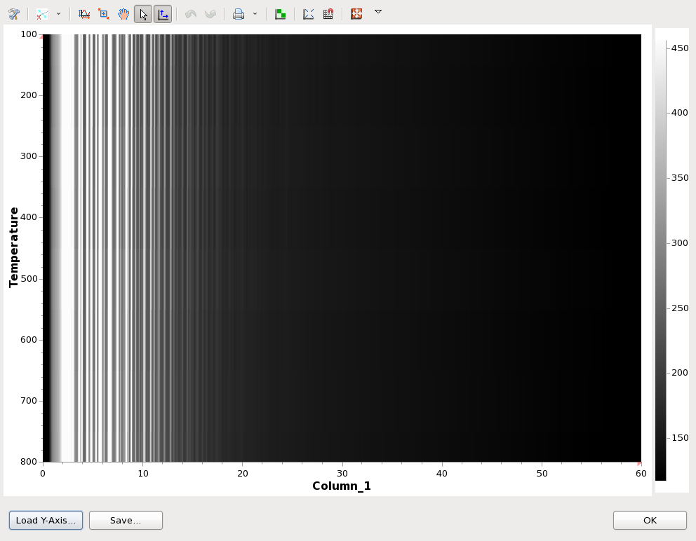
The dialog that appears will show an image where each pattern corresponds to a row of pixels. Clicking the Load Y-Axis... button allows a text file containing the temperature values corresponding to each pattern to be loaded. On loading this data, the y-axis values on the plot should change to reflect this new data.

If everything looks correct the combined data can be saved by clicking the Save... button.

Step 2 - Creating the Fitting Function

Load the combined data file back into DataVis and select to plot the data as a line (the two theta data should automatically be selected as the x-axis).

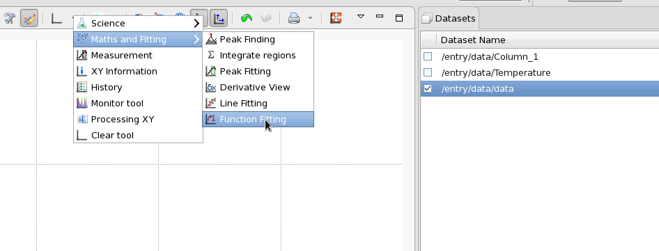
In the plot toolbar, select the xy plotting tools action, and from the drop-down menu, choose Maths and Fitting/Function Fitting. The Function Fitting Tool view will appear (like all views, the tool view can be dragged to a more convenient position if the location it opens in is not ideal) .

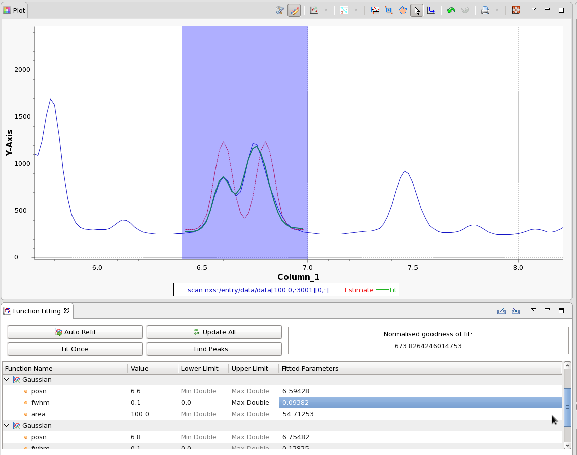
In the plot, adjust the blue region to cover the area of the pattern to be fitted. In this example the doublet between 6.4 and 7 degrees. Zoom in on this region. (Turning off "Rescale plot when plotted data changes" will stop the plot autoscaling whenever new lines are added).

The next step is to build the function. To fit this feature a linear baseline and two Gaussian peaks will be used.

In the Function Fitting tool, click in the table where it says "Add new function" and select Linear. Set the value of the offset, c, to be ~300. The Estimate trace should now show a straight line at the base of the peak.

By the same process, add two Gaussian peaks, give them both a fwhm of 0.1, and area of 100 and positions of 6.6 and 6.8. The Estimate trace should show the combination of the baseline and the two Gaussians.

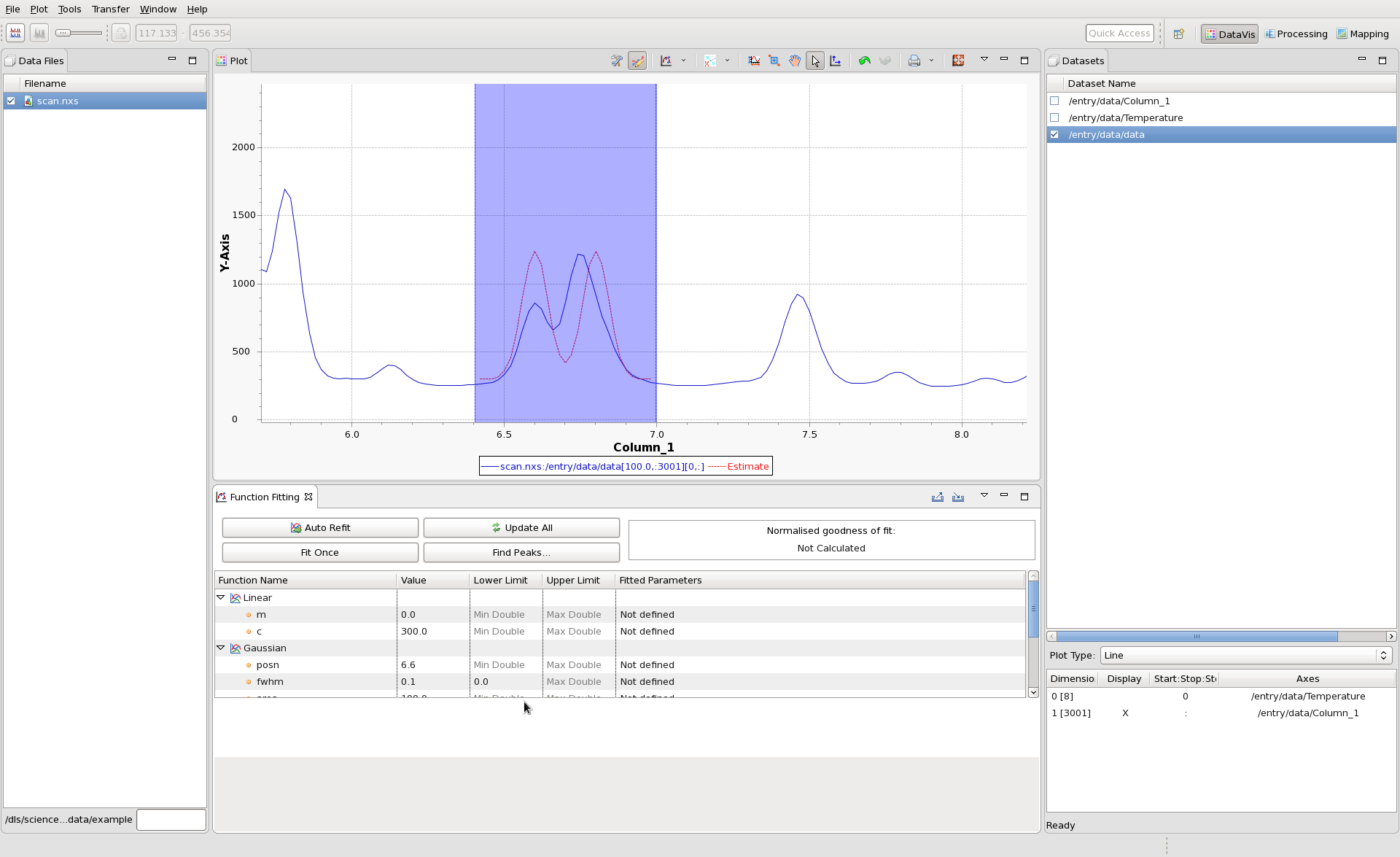
Press Fit Once to optimise the function. Notice how a green Fit trace now appears showing the profile of the function with the optimised parameters. The optimised parameters can be found in the "Fitted Parameters" column. If the optimised fit doesn't accurately reflect the data, try adjusting the input parameters and fitting range (blue box) and fitting again. To fit this function to other patterns in our stack is it possible to use the slicing table (bottom right) to select the next pattern and press fit once again.

It is possible to fit all the patterns in the temperature series by this approach, but it is not very efficient.

To fit this function to the series, the function can be exported to a file, then the Processing perspective can be used to sequentially apply this fit to each pattern. When an function has been defined that optimizes correctly, in the Function Fitting tool toolbar, click the Export function button, and save the function to file.

Step 3 - Fitting the Function To the Series

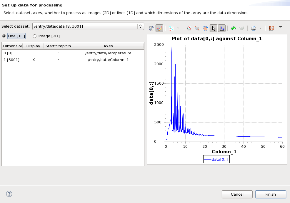
Switch to the Processing Perspective, and load the combined file. In the dialog that appears, select to processing the combined data (/entry/data/data [8,3001]), as a Line (the Column_1 and Temperature axes should be picked up automatically).

Once loaded, the first pattern should be shown in the Input view. Click in the Processing view table and add Fit Imported Function (typing fit should filter out the other processing steps). In the Model view table, click in the Value column next to Function File, and file browser to select the saved function file created earlier. Click back on the Fit Imported Function entry to update it with the new path. When the process runs, the data should be visible in the Output view, with the fitted function and residual traces.

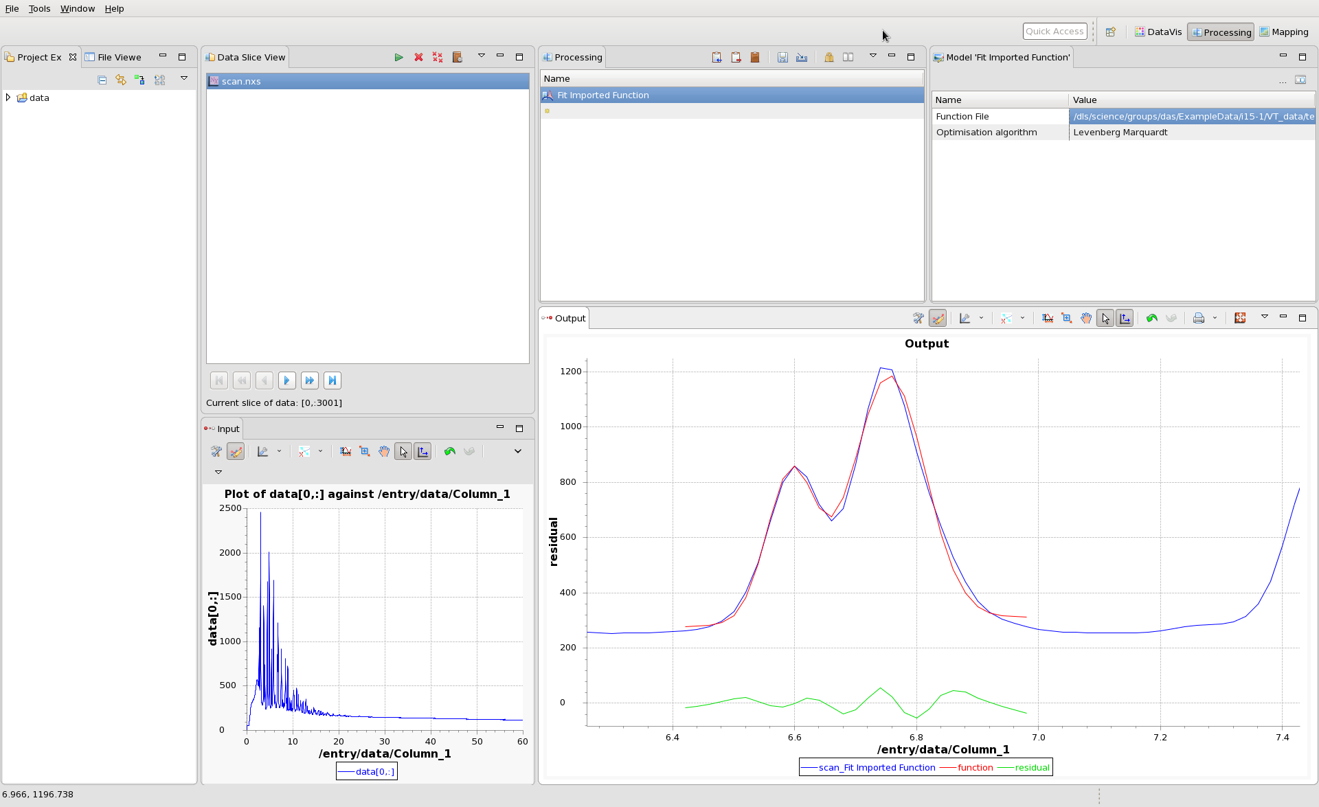
Pressing the green play button at the top of the Data Slice View, will process all the data, saving the output parameters out into a Nexus file.

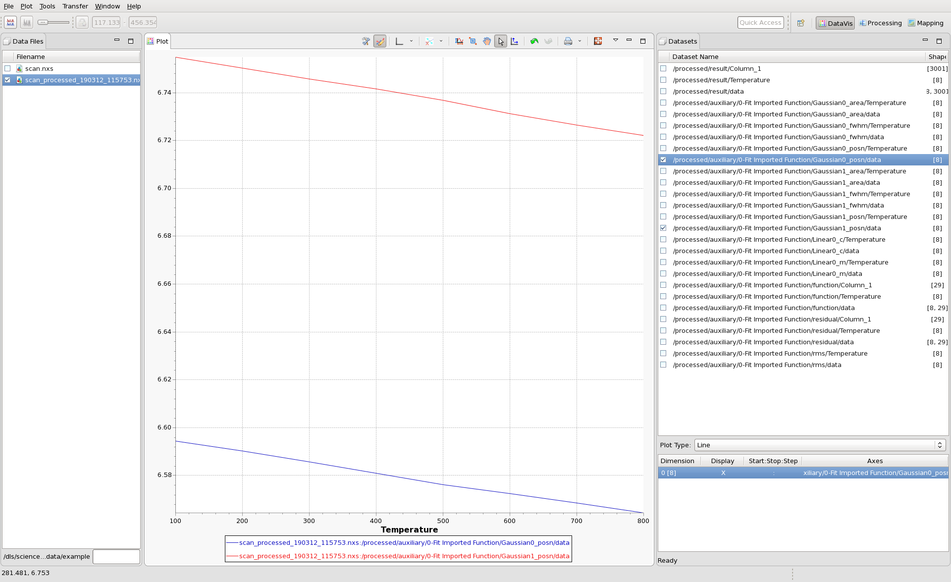
Opening the output Nexus file in DataVis allows the fitted parameters to be plotted as a function of Temperature.