...
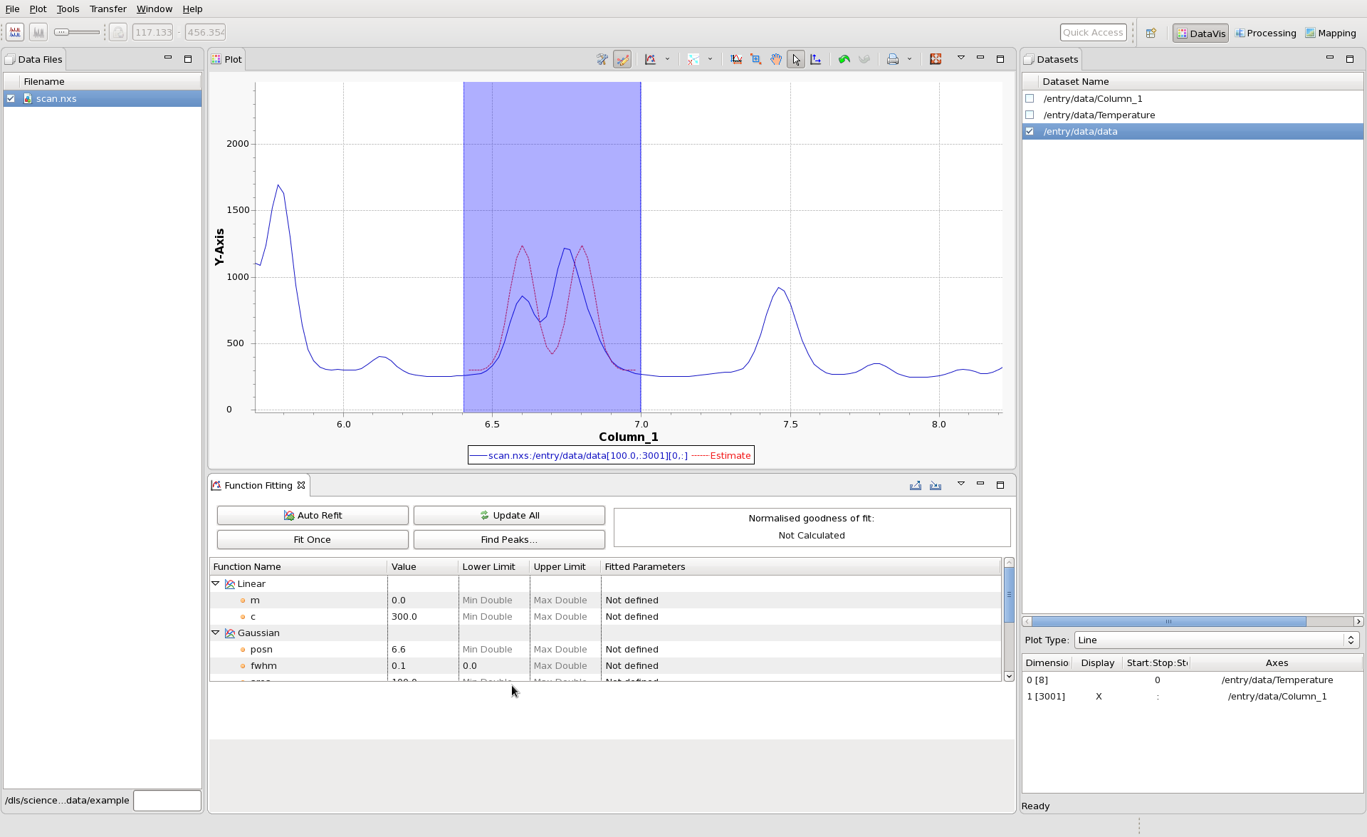
In the plot, adjust the blue region to cover the area of the pattern to be fitted. In this example the doublet between 6.4 and 7 degrees. Zoom in on this region. (Turning off "Rescale plot when plotted data changes" will stop the plot autoscaling whenever new lines are added).
The next step is to build the function. To fit this feature a linear baseline and two Gaussian peaks will be used.
In the Function Fitting tool, click in the table where it says "Add new function" and select Linear. Set the value of the offset, c, to be ~300. The Estimate trace should now show a straight line at the base of the peak.
By the same process, add two Gaussian peaks, give them both a fwhm of 0.1, and area of 100 and positions of 6.6 and 6.8. The Estimate trace should show the combination of the baseline and the two Gaussians.
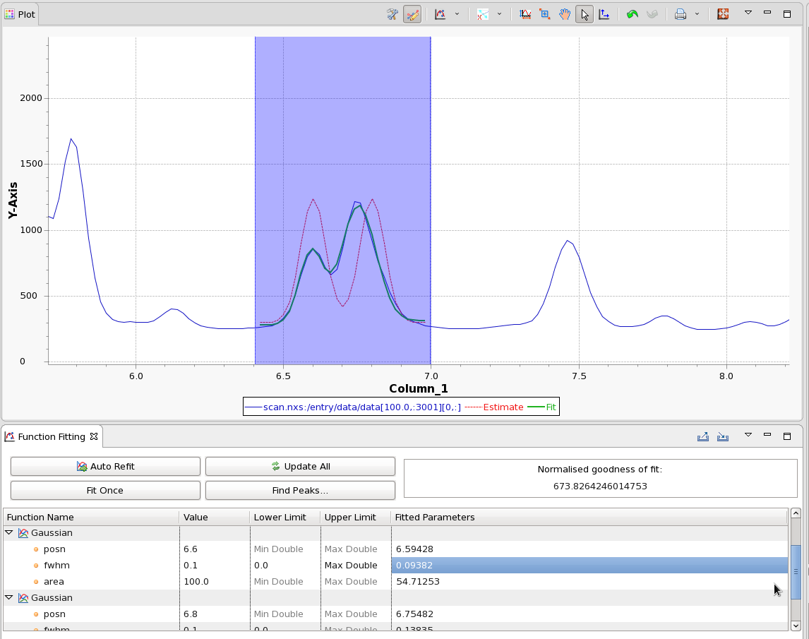
Press Fit Once to optimise the function. Notice how a green Fit trace now appears showing the profile of the function with the optimised parameters. The optimised parameters can be found in the "Fitted Parameters" column. If the optimised fit doesn't accurately reflect the data, try adjusting the input parameters and fitting range (blue box) and fitting again. To fit this function to other patterns in our stack is it possible to use the slicing table (bottom right) to select the next pattern and press fit once again.
 It is possible to fit all the patterns in the temperature series by this approach, but it is not very efficient.
To fit this function to the series, the function can be exported to a file, then the Processing perspective can be used to sequentially apply this fit to each pattern. When an function has been defined that optimizes correctly, in the Function Fitting tool toolbar, click the Export function button, and save the function to file.