Introduction

This quick start guide is a rapid tour through the three main generic perspectives in DAWN, DataVis, Mapping and Processing.

The guide uses a NeXus (tagged HDF5) file containing a few different datasets which can be downloaded from here https://alfred.diamond.ac.uk/DawnExampleData/ftir1.nxs

This file is from a Infrared imaging experiment of a fixed cell sample, and is a nice example since it can be visualised in many different ways.

Lets get started...

If you haven't already, download the example data file from here: https://alfred.diamond.ac.uk/DawnExampleData/ftir1.nxs

To get a copy of DAWN go to www.dawnsci.org/downloads and download the correct version for your operating system. If you download DAWN as a zip file it needs no installation, just unzip the file into a suitable location and double-click on the dawn executable to start.

(If you are on a Linux workstation in the Diamond Light Source, the latest version of DAWN can be obtained by typing "module load dawn", in the command-line then pressing enter, followed by "dawn".

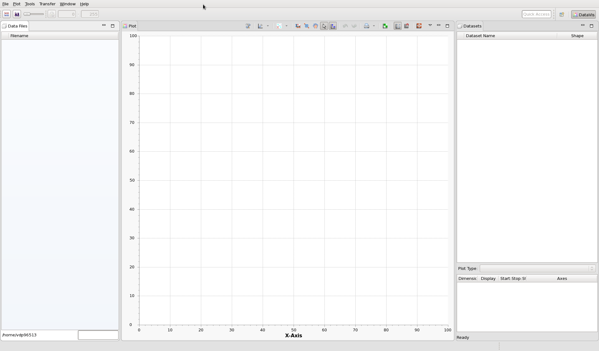
You should see the splash screen, then DAWN will start, and should look something like this:

(DAWN stores its state when you close it down, so if this is not what your DAWN looks like, its possibly because you have started it before. If you want to reset everything and completely start from the beginning follow the instructions at the bottom of the page).

Loading and Viewing Data - DataVis

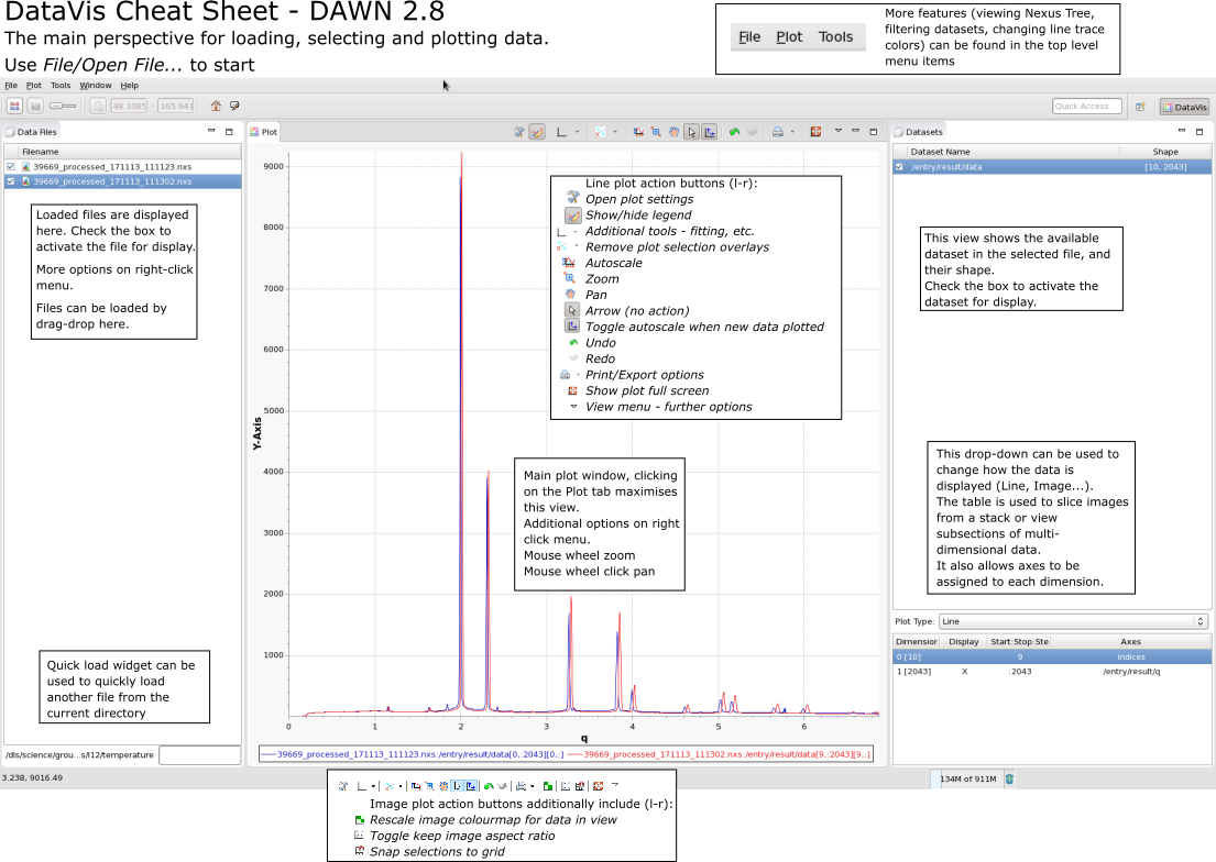
By default DAWN starts up in the DataVis perspective (for more on perspectives see here #TODO insert link). The main purpose of this perspective is to allow data from multiple files to be viewed in multiple different ways.

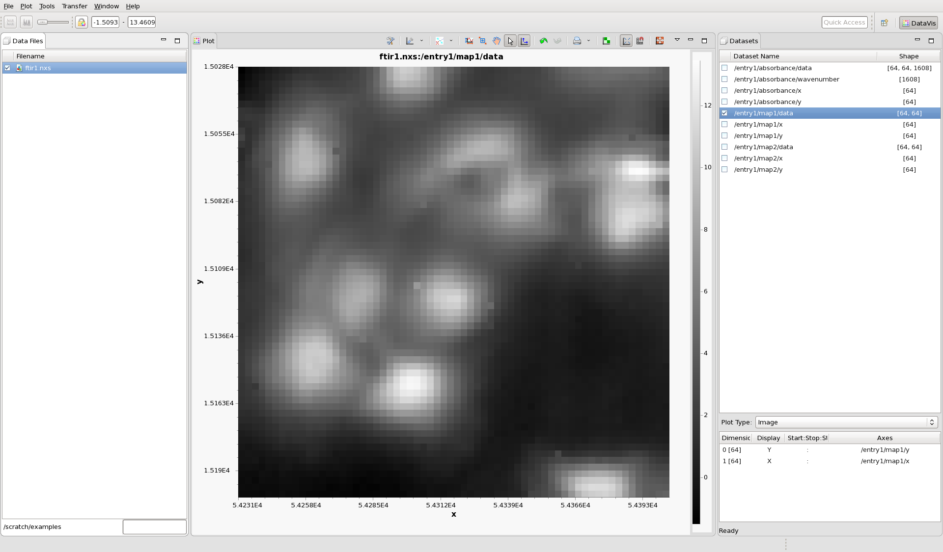
In the main File menu, select Open File... and select the NeXus file you have just downloaded. Check the box next to the filename ftir1.nxs to display some data from the file (DataVis uses the tagging in the NeXus file to choose which dataset to show by default). It should look like this.

DAWN has selected to plot /entry1/map1/data as an image (it is an infrared image of some cells). Different datasets can be plotted by checking the box next to the name of the dataset in the Datasets view. Check the box next to /entry1/map2/data to see this image (the same cells at a different wavelength).

By default, datasets with two or more dimensions are plotted as images, 1D data is plotted as a line. Check the box next to /entry1/absorbance/wavenumber. This is 1D, so is plotted as a line.

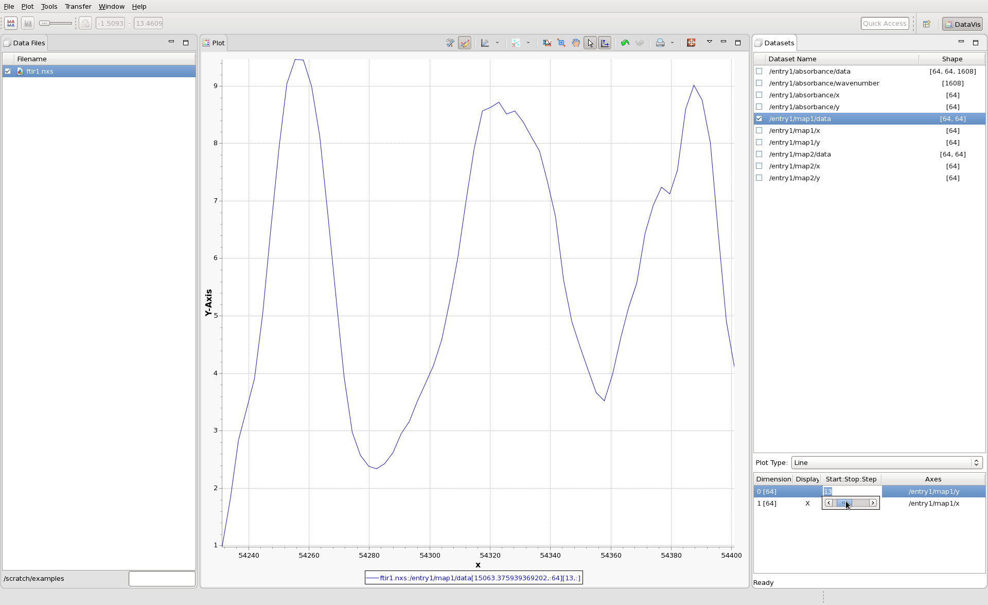
It is possible to view higher dimensional datasets as lines. Plot /entry1/map2/data again, and in the Plot Type drop down box (which currently shows image) select line. See how the first row of the image is now shown as a line. Different rows (or slices) of the image can be shown by changing the Start:Stop:Step value in the Dimension table. In this table, click in the Start:Stop:Step column for Dimension 0 [64], a slider will appear to let you scroll through the rows. Alternatively a specific row can be selected by typing in the row index.

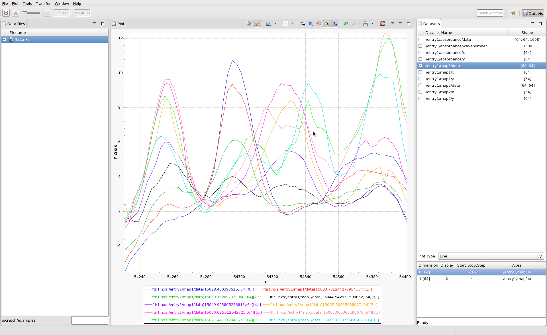
To view multiple rows of the image, as lines, at the same time, enter a start:stop:step slice in the box. For example entering 0:20:2 will show you every other row, starting from zero, up to 20 (exclusive - 20 will not be shown). It should look like this.

When taking multiple lines like this, it is still possible to use the slider to slice through the dataset, it just changes the start and stop indices, keeping a constant step.

To view the columns of the image instead of the rows, in the Display column of the Dimension table, click in the cell next to Dimension 0 [64] and select X from the drop down box that appears. The columns can be sliced in the same manner as the rows.

When displaying these image and line plots, you may have noticed that the x and y axes had values ~15000 for y and ~50000 for x, these are position on the cell image in microns, on the IR microscope stage. They have been automatically selected due to the tagging in the NeXus file. Clicking on the cell in the Axes Column of the Dimension table will show you all the axes available to plot. Selecting indices (the default when there is no tagging), plots the data against its index position in the data array (0-63 for /entry1/map1/data).

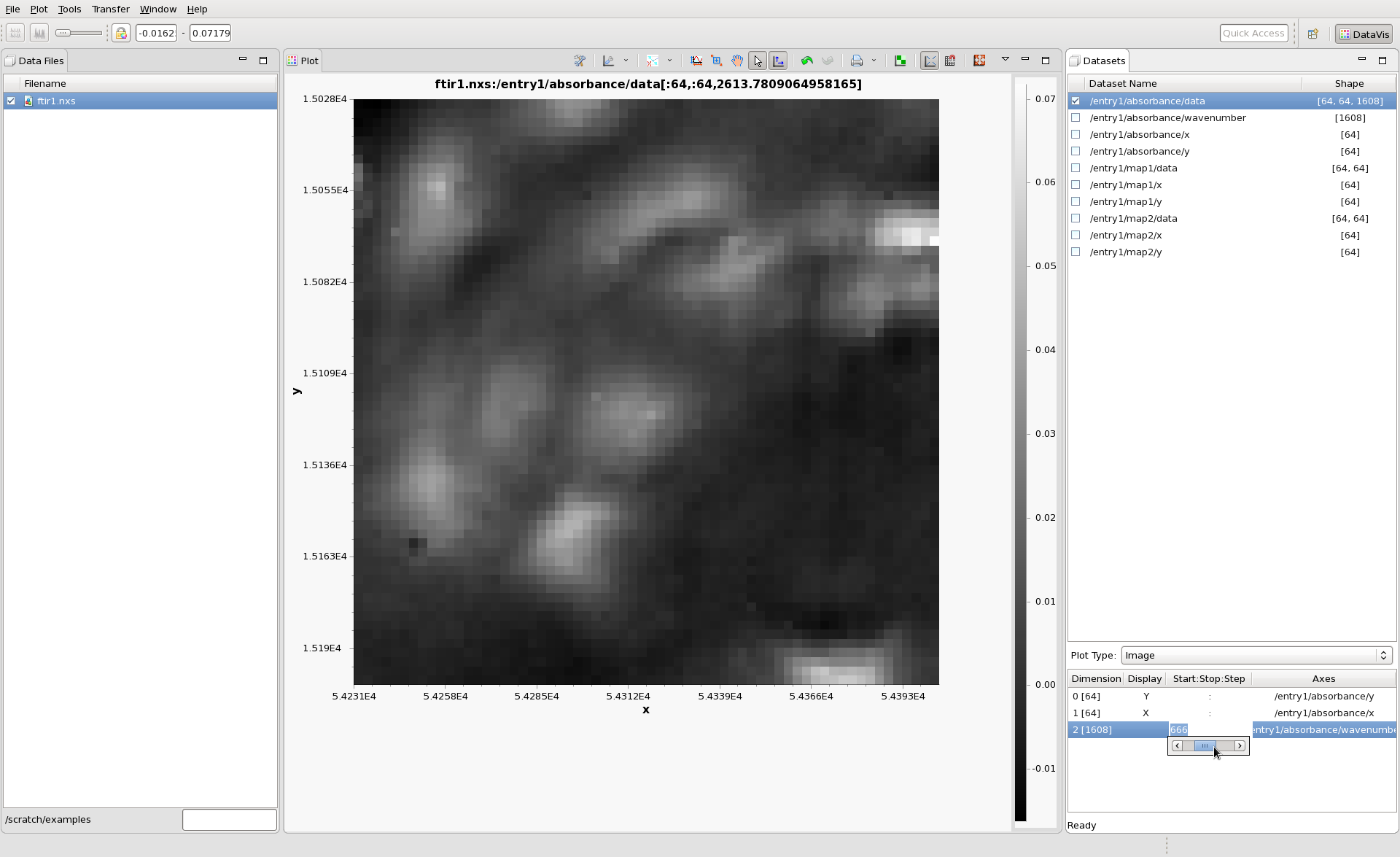
Finally, check the box next to /entry1/absorbance/data. It is a 3D dataset with shape [64,64,1608] (for this measurement it is 1608 64x64 images, taken a different wavelengths in the Infrared, alternatively expressed as a 64x64 grid of Infrared spectra). Using DataVis, you should be able to configure the Plot Type and Dimension table to show this dataset as a 64x64 image, then slice down the 1608 wavelengths using the slider, like this:

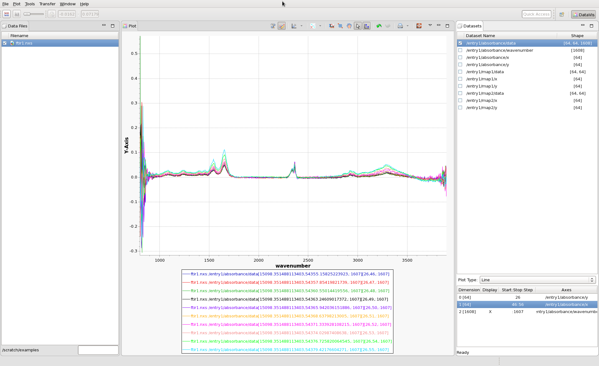
It is also possible to view the data as spectra, by displaying lines, with the 1608 dimension as X, like this:

Using this dataset, try some of the other modes in the Plot Type drop down and see what happens. More information on the DataVis perspective can be found here #TODO link.

Loading and Viewing Data - Mapping

The data file used in this example contains several datasets composed of values taken at different spatial location in a sample. For data collected like this (a grid scan of an area detector, or array detector for example), and is stored in a NeXus file that meets certain criteria, the Mapping Perspective in DAWN can be used to view this data in a more intuitive way.

To open the mapping perspective:

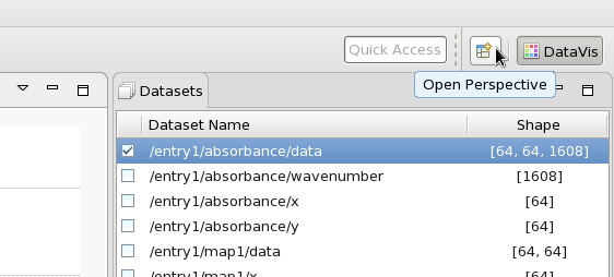
Click the Open Perspective button in the top right corner of the main window.

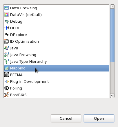
From the dialog that opens, select Mapping and click Open.

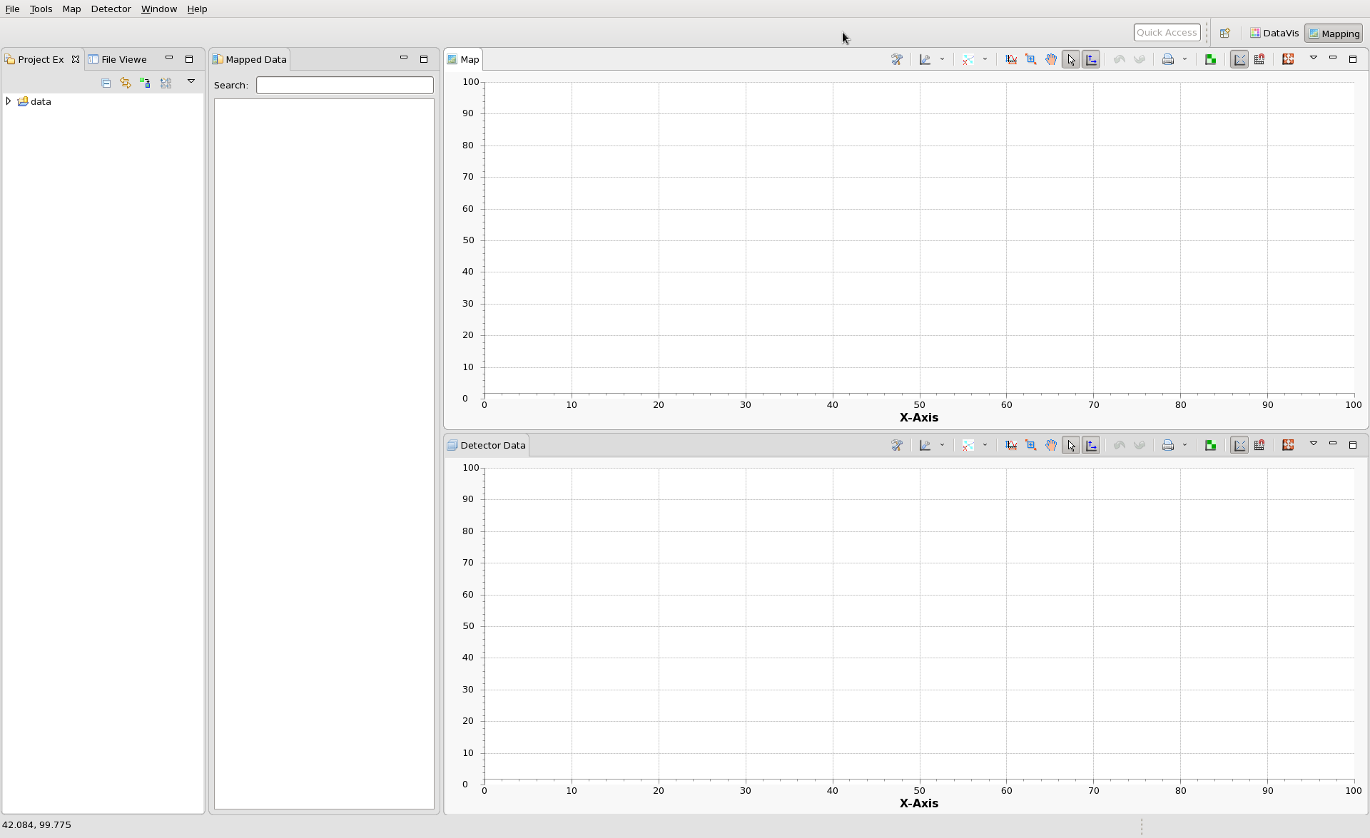
The main window will then switch to the Mapping Perspective. It should now look like this:

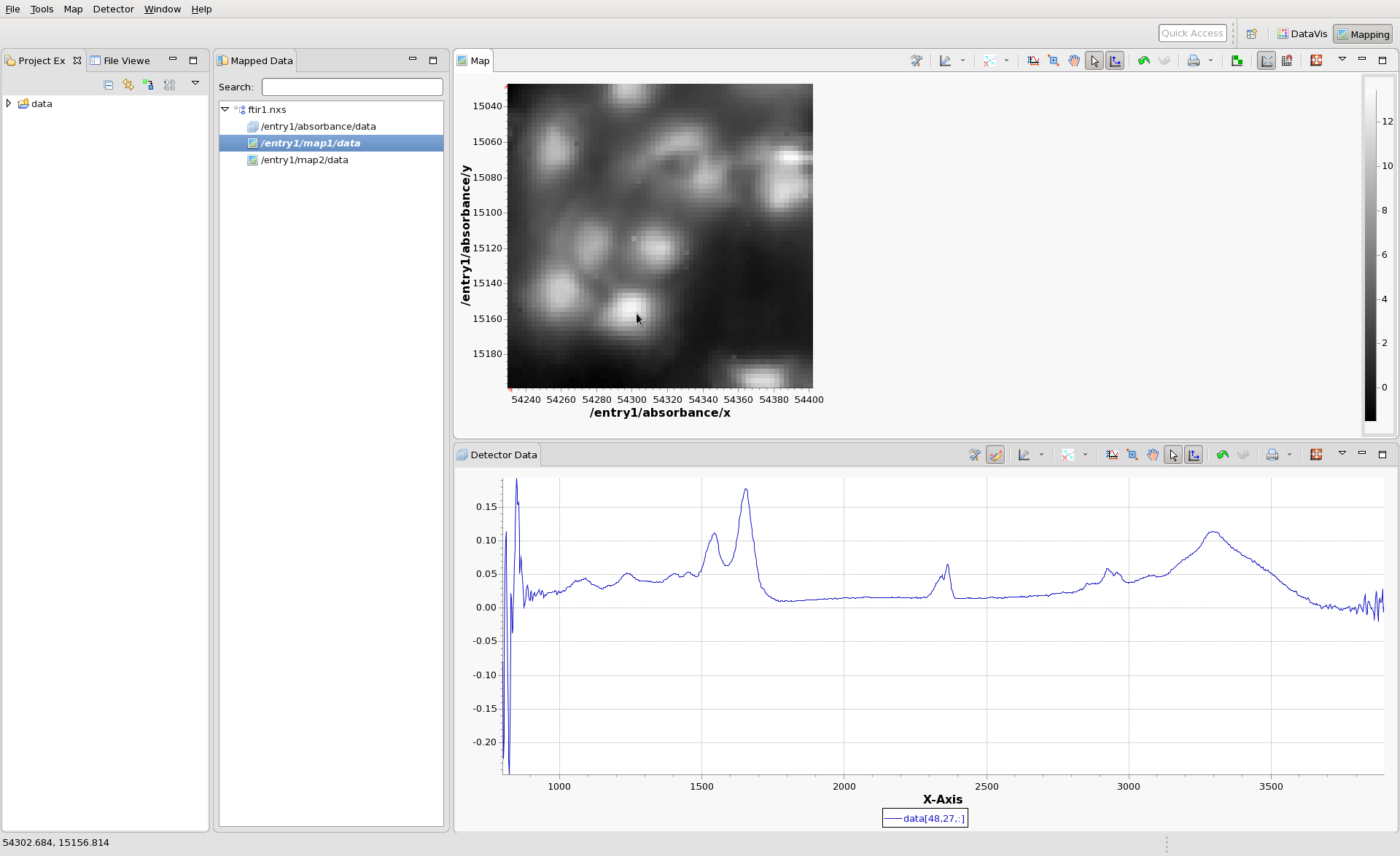
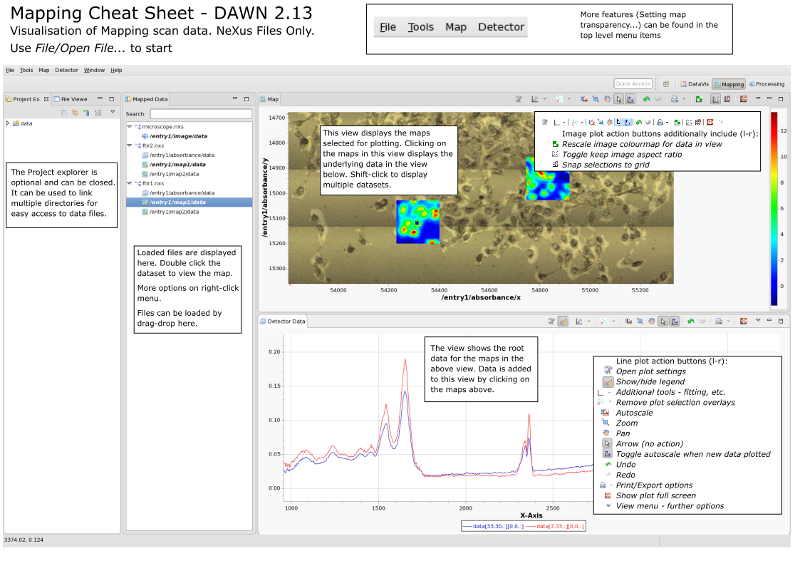
Again open the ftir1.nxs file (again using File/Open File or using File/Recent Files if this was recently loaded into DataVis). In the Mapped Data View, make sure the ftir1.nxs tree node is expanded and double click /entry1/map1/data, then do a single click somewhere on the image that appears. You should have something that looks like this:

When you click on a pixel in the cell image, the mapping perspective shows you the Infrared spectrum that corresponds to that pixel (recall the absorbance dataset is 3D, with one 1608 point IR spectrum per pixel, with 64x64 pixels in the image).

When a file is loaded into the mapping perspective, it parses the file structure and determines what datasets can be displayed as images (the maps in this case) and what are the higher dimensional datasets that should be displayed when the map is clicked on. The map being viewed can be changed by double clicking a different map option in the Mapped Data View. Double click on /entry1/map2/data to view this map.

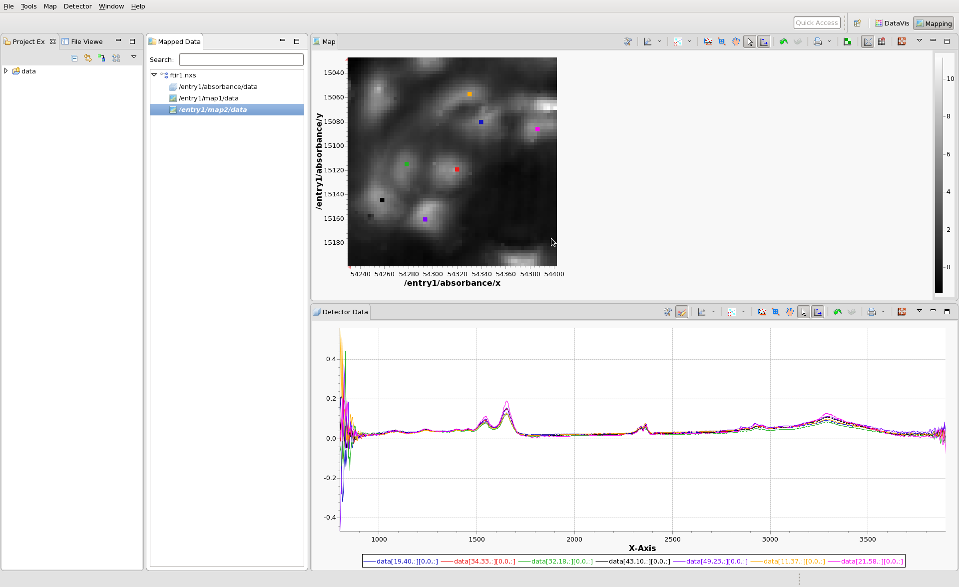
It is possible to view multiple spectra from different locations of the image at the same time. Hold shift, then click in the Map view on the image. Every time you click a coloured marker is put down and another spectrum is added to the Detector Data View.

This is very similar to the slicing of data in the DataVis perspective seen earlier, but is a much more useful and intuitive way to view this kind of data. It is possible to load multiple files into the mapping perspective, allowing data from different files, but measured on the same sample, to be compared directly. More information on how to use the mapping perspective can be found here #TODO add link to mapping perspective guide

Processing Data - Processing

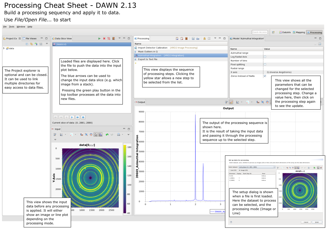
In the last part of this quick start guide we will consider how to process data. The Processing Perspective in DAWN is designed to take data (either 2D images or 1D spectra/patterns/traces) and pass it through a series of processing steps. These processing steps can then be applied to every image in the stack (or 1D spectrum in a 3D block etc).

In the same way you switched to the mapping perspective, now switch to the Processing, and again load ftir1.nxs.

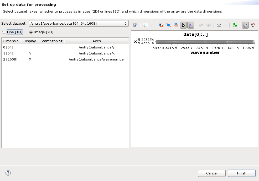
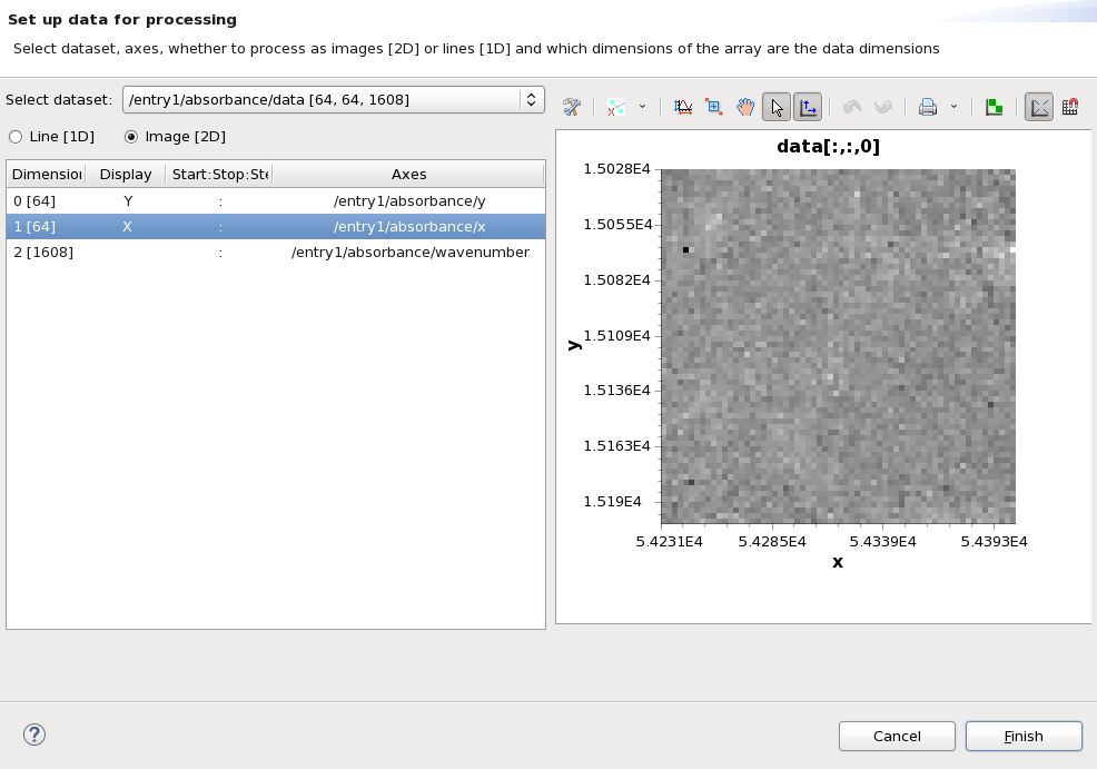
This time, loading the file will open a dialog for setting up the data for processing. It should look like this.

The processing perspective can only process one dataset from a file at a time, before we can use the perspective we need to select which dataset (in this case /entry1/absorbance/data) and how we want to slice it for processing (in this case as a 64x64 image). Make sure /entry1/absorbance/data is in the select dataset drop down, Image [2D] is selected and Dimensions 0 [64] and 1 [64] are selected to display X and Y. The dialog should now look like this:

We are going to process the stack of 64x64 IR images. Click the Finish button.

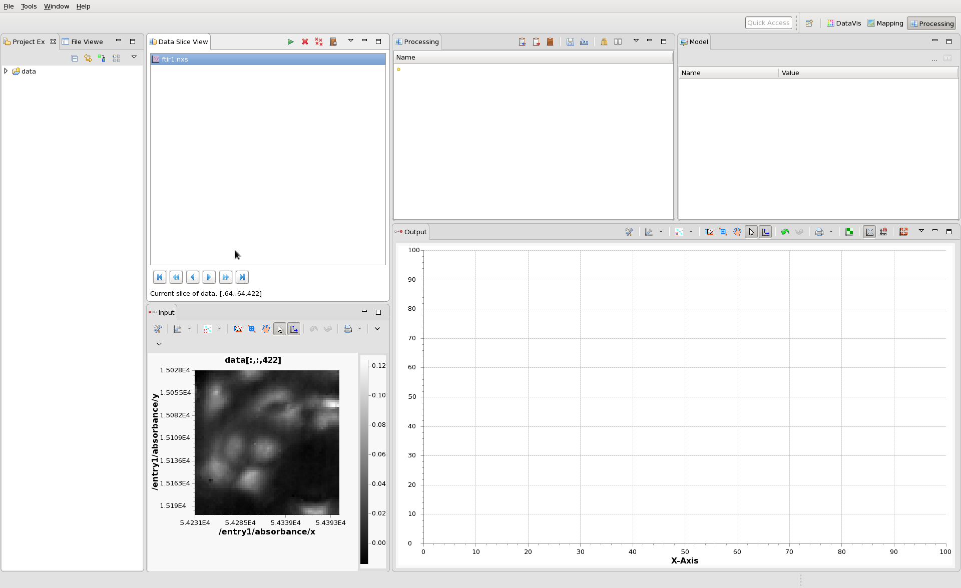
The Processing perspective should show ftir1.nxs in the Data Slice View and the first image in the Input plot. The image shown in the input can be changed using the blue play/fast forward buttons at the bottom of the Data Slice View. Click these buttons and see how the input image changes.

Now we can start to build our processing chain. In the Processing View, click the small yellow star and type ga. From the drop down that appears select Gaussian Filter.

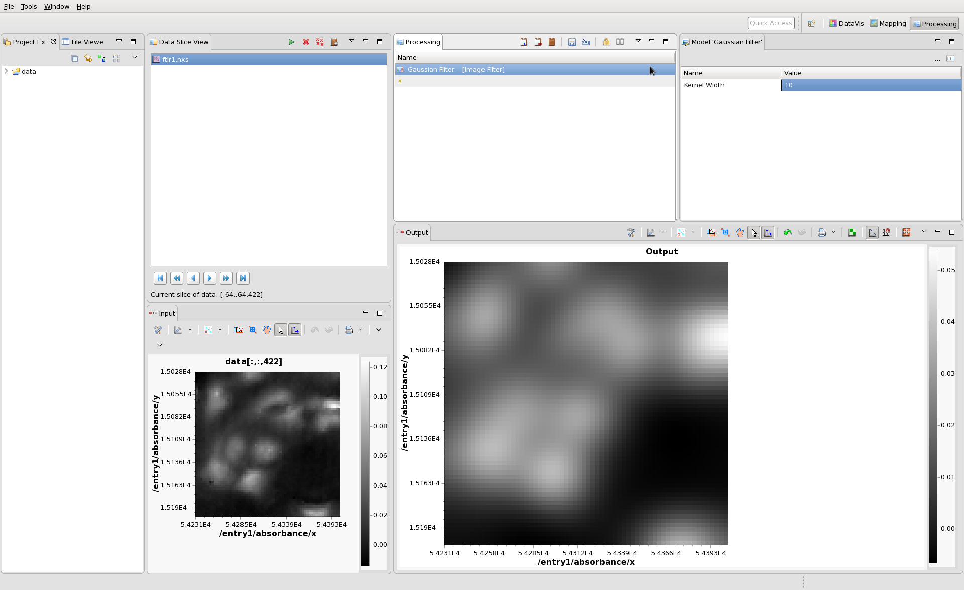
The Input image is then passed through the Gaussian Filter and the result is plotted in the Output view. The Model view shows all the parameters of the Gaussian Filter that can be adjusted. Change the Kernel Width to 10 then click back on the Gaussian Filter entry in the Processing view to update the Output. It should look something like this:

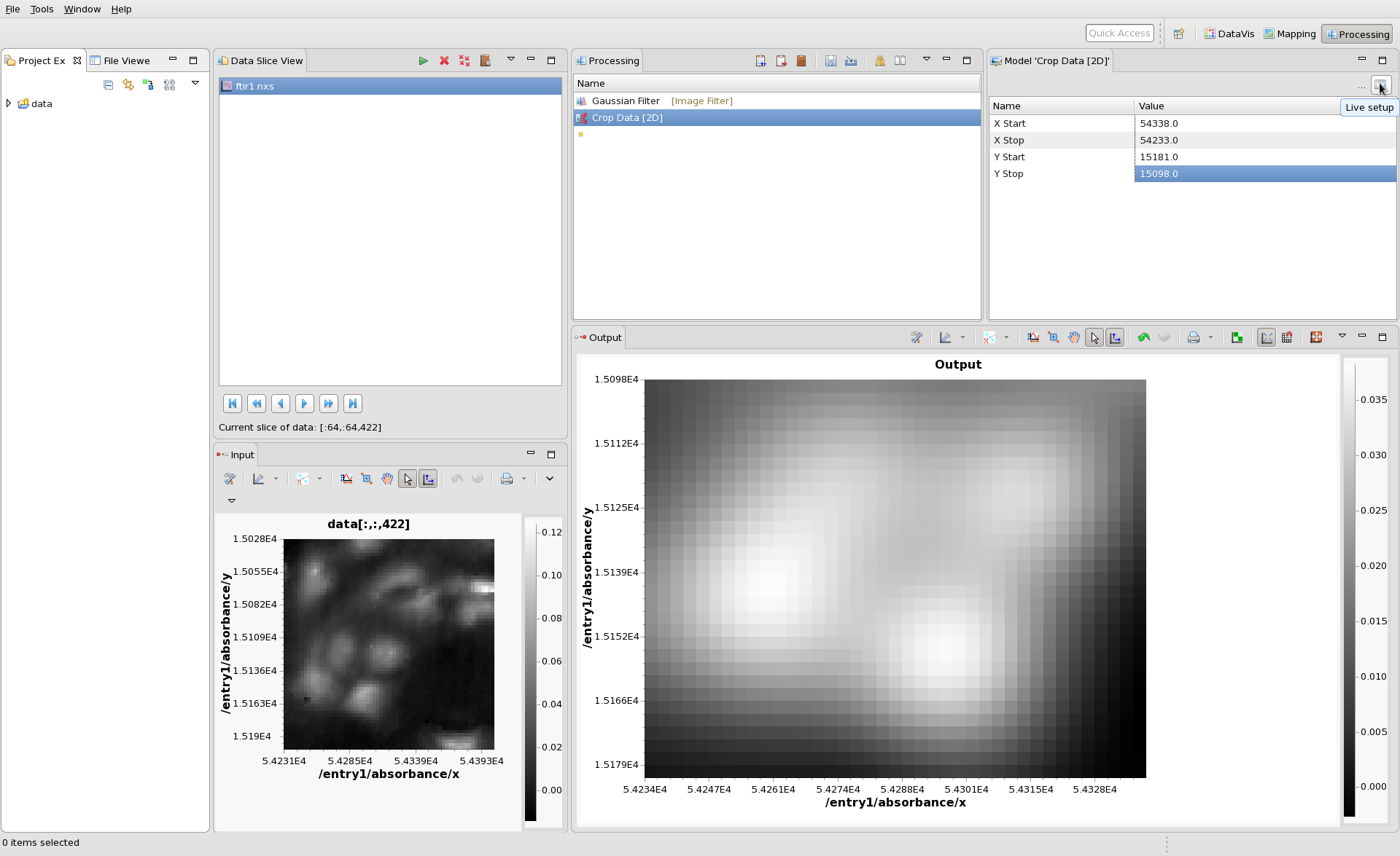
Next add Crop Data [2D] as a processing step. This step can be used to crop the image. The Crop Model has boxes where the X and Y start and stop for cropping can be entered (remembering for this dataset X and Y have micron values from the sample stage). Entering sensible values and clicking back on the Crop Data entry should show the blurred, cropped data in the output.

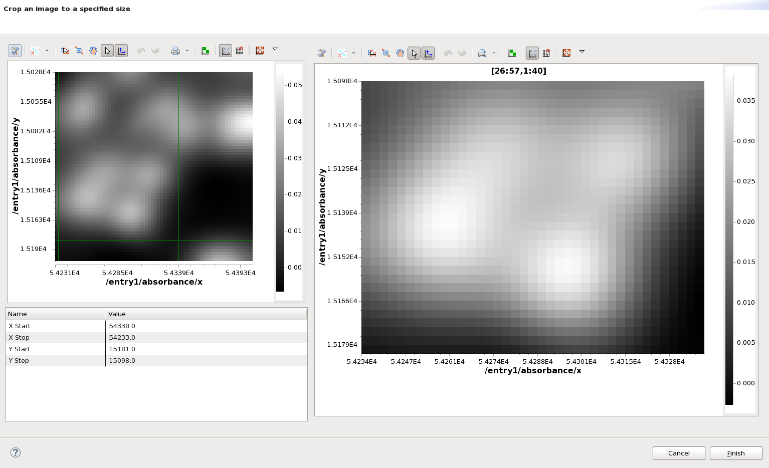
For processing steps like the Crop, entering these values by hand can be a bit awkward. The Model View has a Live Setup dialog to help in these cases. Click the live setup button (top right button in the Model view), and the Live Setup dialog will appear.

The Crop Start and Stop values can now be set by dragging the green lines plotted on the image on the left (they may be at the very edge of the plot if you cant see them initially). Once you are happy click Finish and then click the Crop step in the Processing view to update the output.

Now the processing sequence is complete pressing the green play button at the top of the Data Slice View will apply this processing to all the images in the stack, writing the result to a new NeXus file. In the dialog that appears, select the directory to process the data into. You can also check Automatically load data to DataVis perspective, if you want to view the results when the process has finished (you will need to manually switch back to DataVis).

Instead of processing this dataset as images, the Processing perspective can also be used to process the dataset as a block of spectra. Try unloading the file (red cross button at the top of the Data Slice View), then loading it again, then using the setup dialog to set the processing to Line [1D] with Dimension 2 [1608] as X. See if you can use a Crop step to cut out the noisy data at the ends of the spectrum.

 More information on the Processing Perspective can be found here #TODO link to processing perspective guide.

Cheatsheets

The Cheatsheets are a single page with a brief guide to each perspective.

DataVis

Mapping

Processing

Troubleshooting

#TODO reseting perspectives, reset workspace, deleting workspace.