ARPES Data Reduction

In this training we will work through the process of reducing some arpes data using a gold calibration sample which is shown in this movie, and the following document.

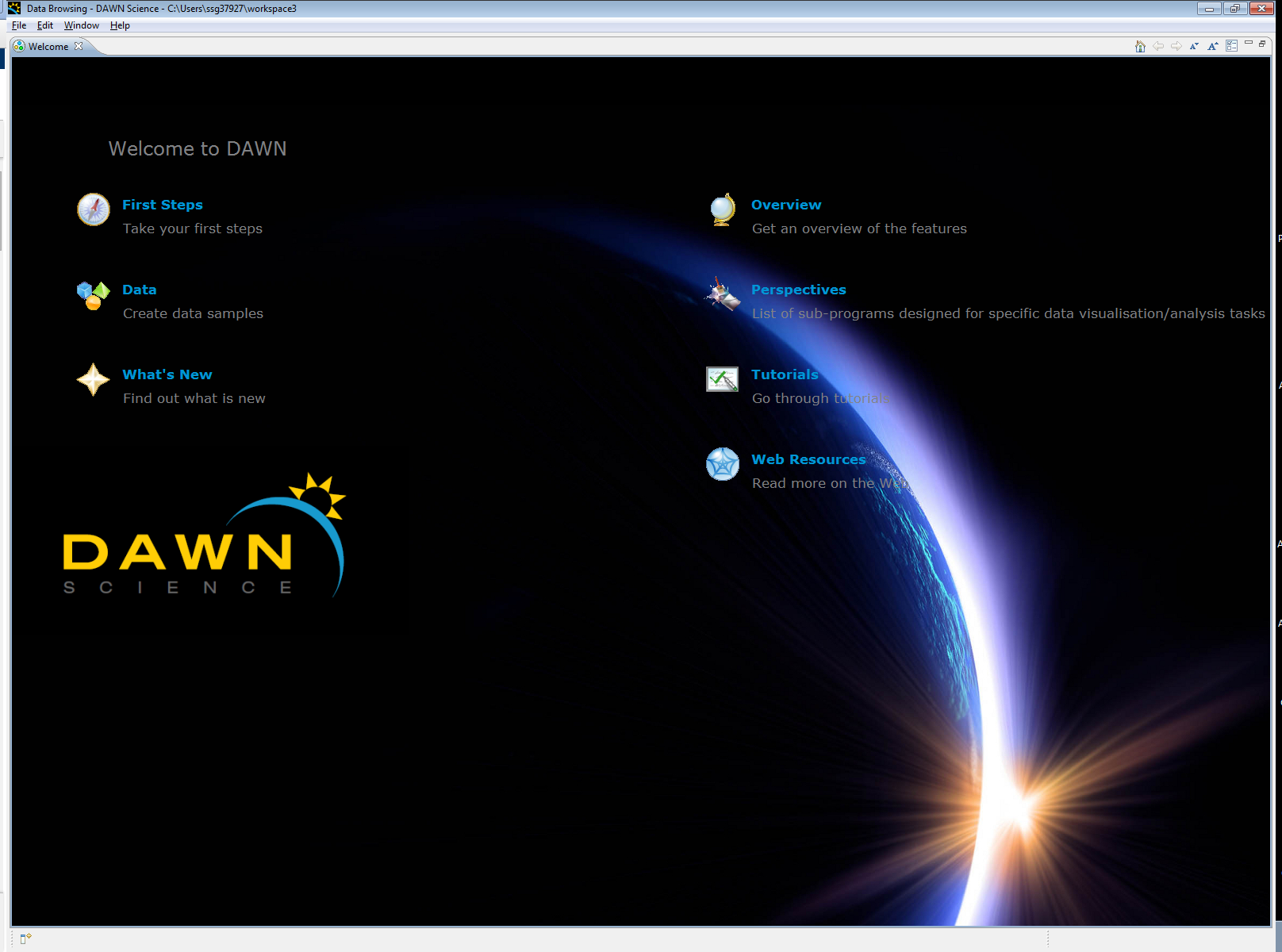
Starting DAWN

In Linux Open a terminal and type

module load dawn

dawn

Or in windows double click the dawn executable

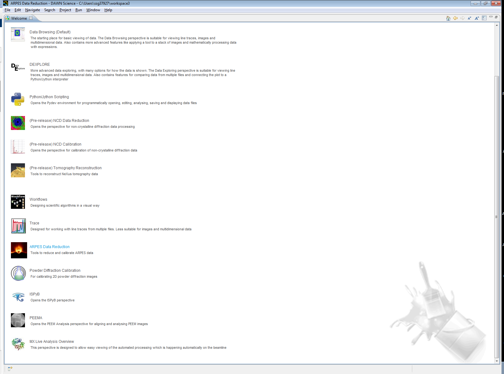
Opening the ARPES Perspective

Select the perspectives option

Then select the Arpres Perspective

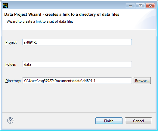
Now add a link to your data as prompted, and click finish.

Preparing the gold calibration file

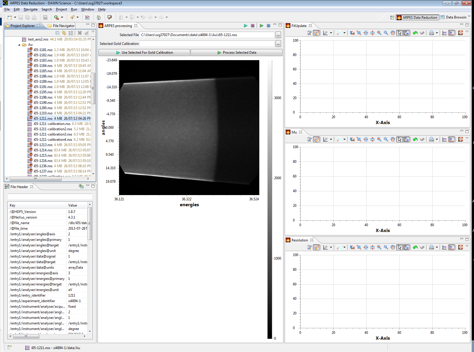
Select an appropriate gold calibration scan (just by single clicking on it), and click the "Use selected for Gold Calibration" button

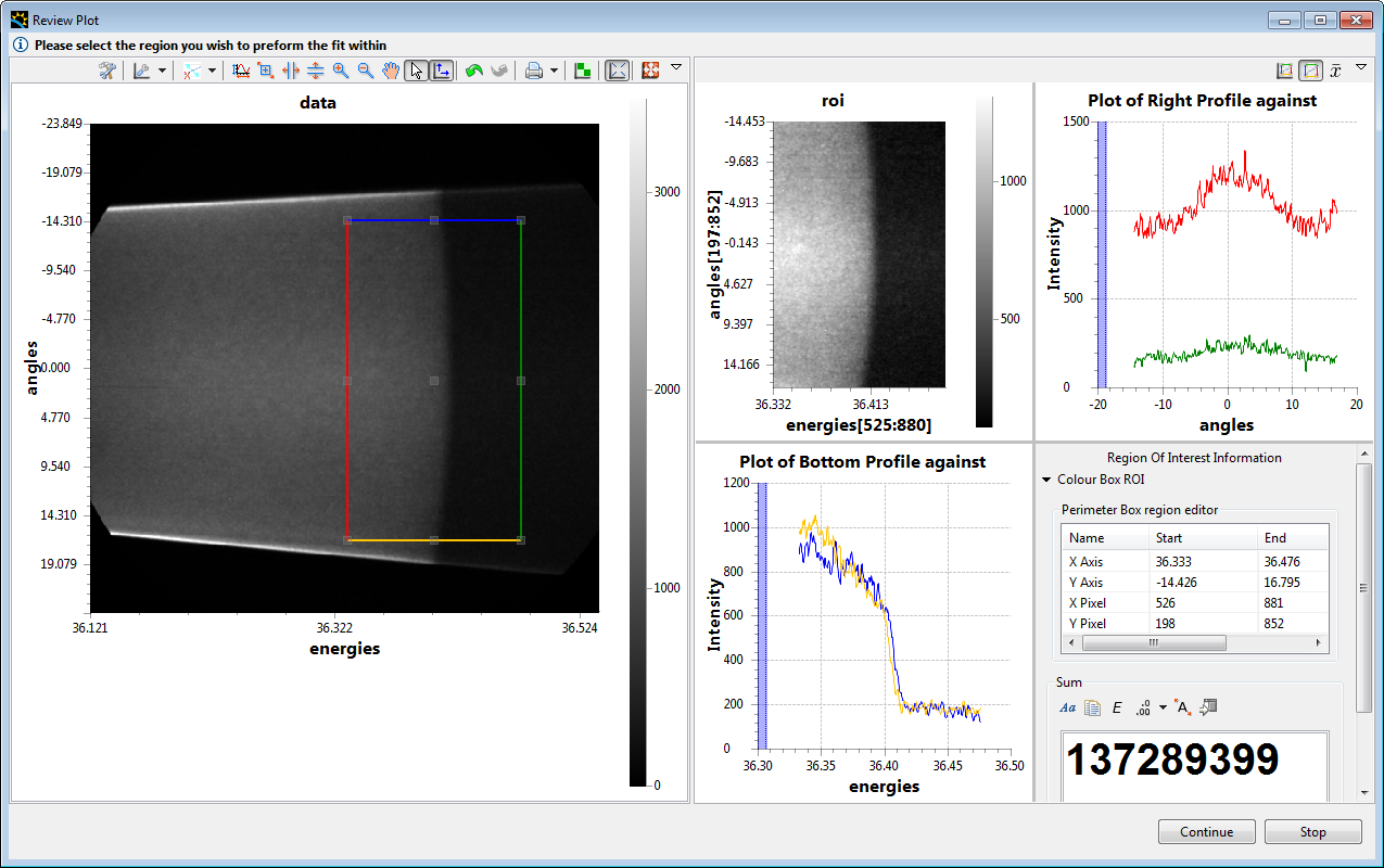
Select a region to fit the fermi egde within, and click continue

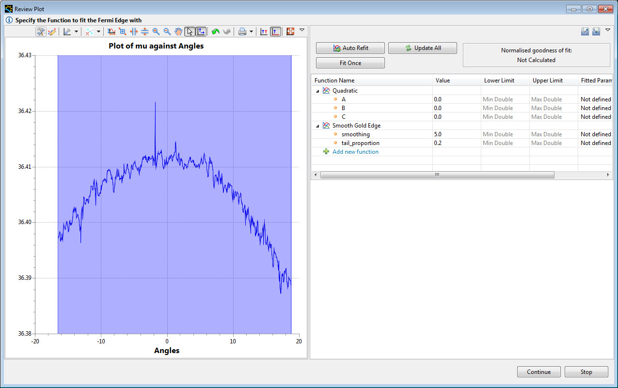
The fit will give you some initial parameters.

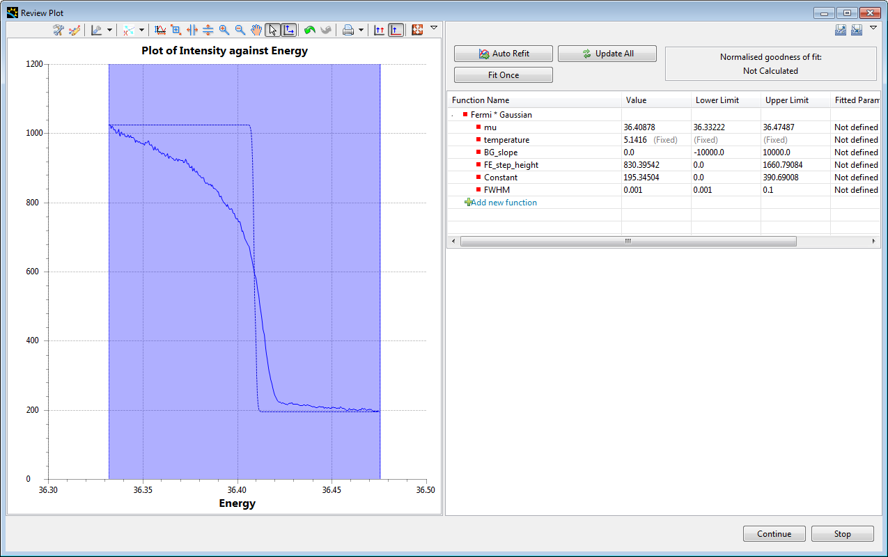
 Change these, and use the fit one, or the auto refit buttons to refine the fit you want to use, then click continue.

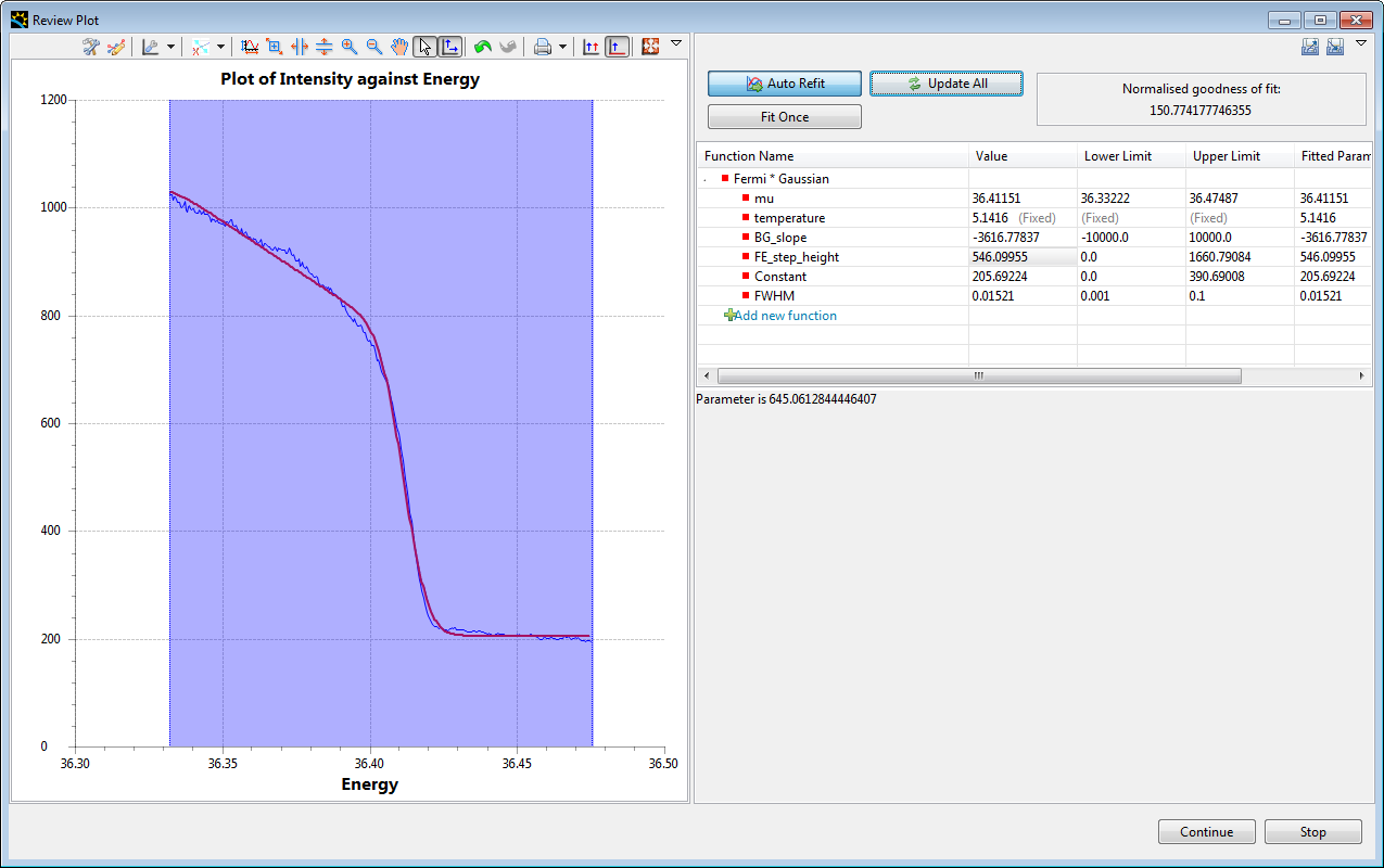
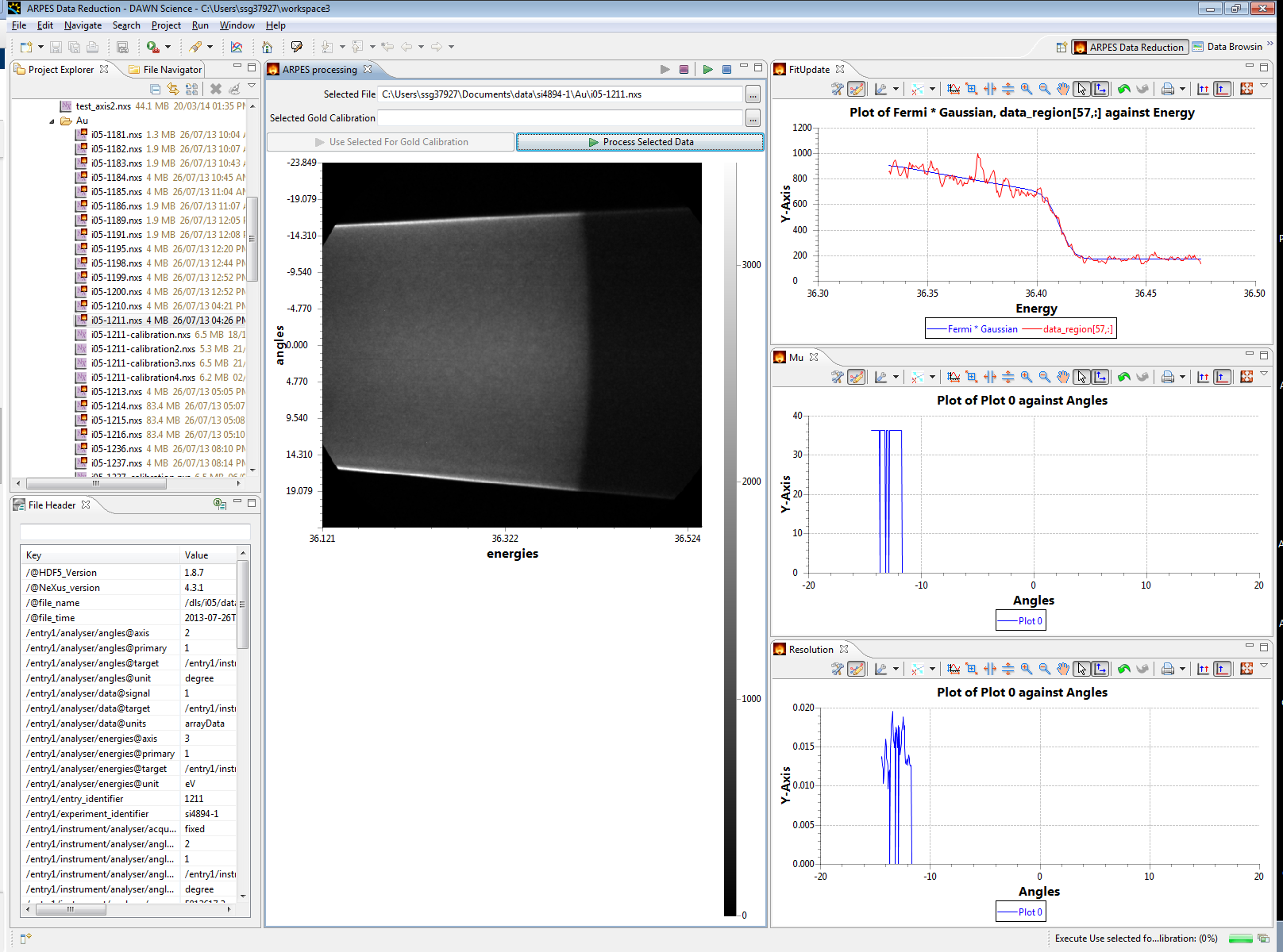
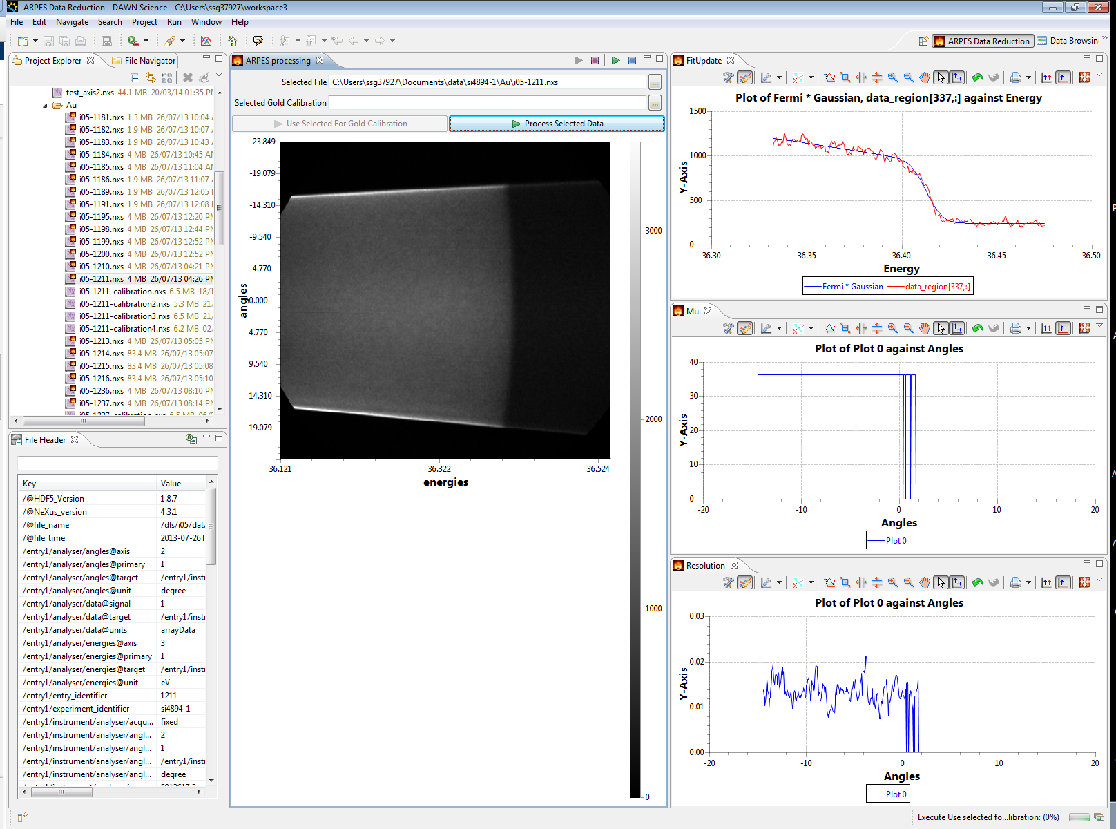
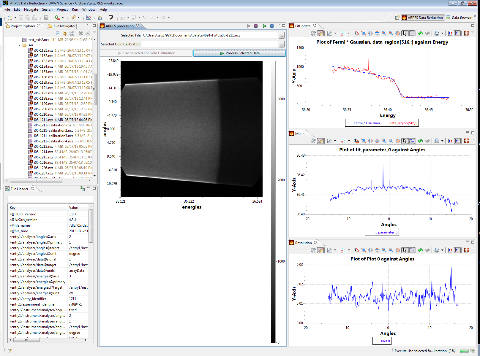
You should then be able to see the fitting progress

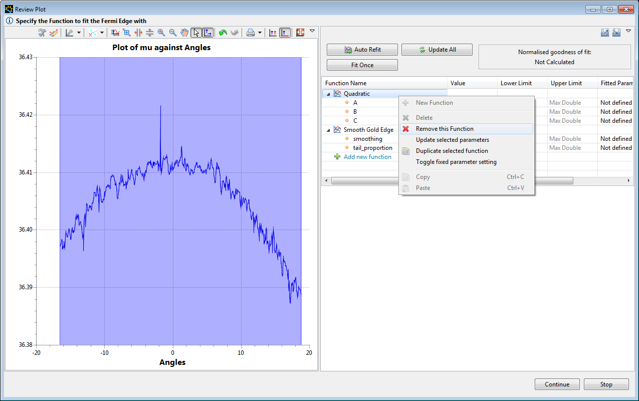
You now have a choice to fit either a Quadratic Function, or a Smoothed function through the gold edge.

To do this select the function you do not wish to use and remove it, for example if you want to use the smoothed gold select the Quadratic function and remove it.

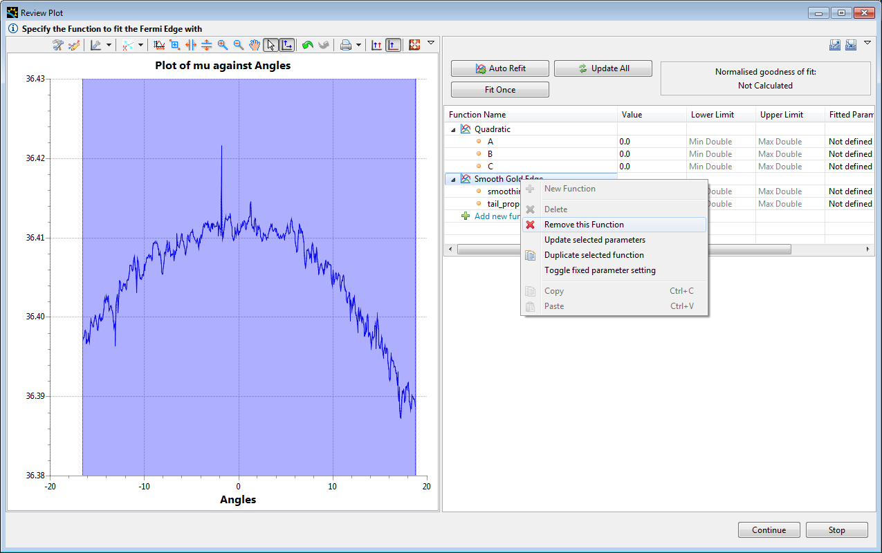
OR if you want to use the quadratic function, right click and remove the Smoothed function

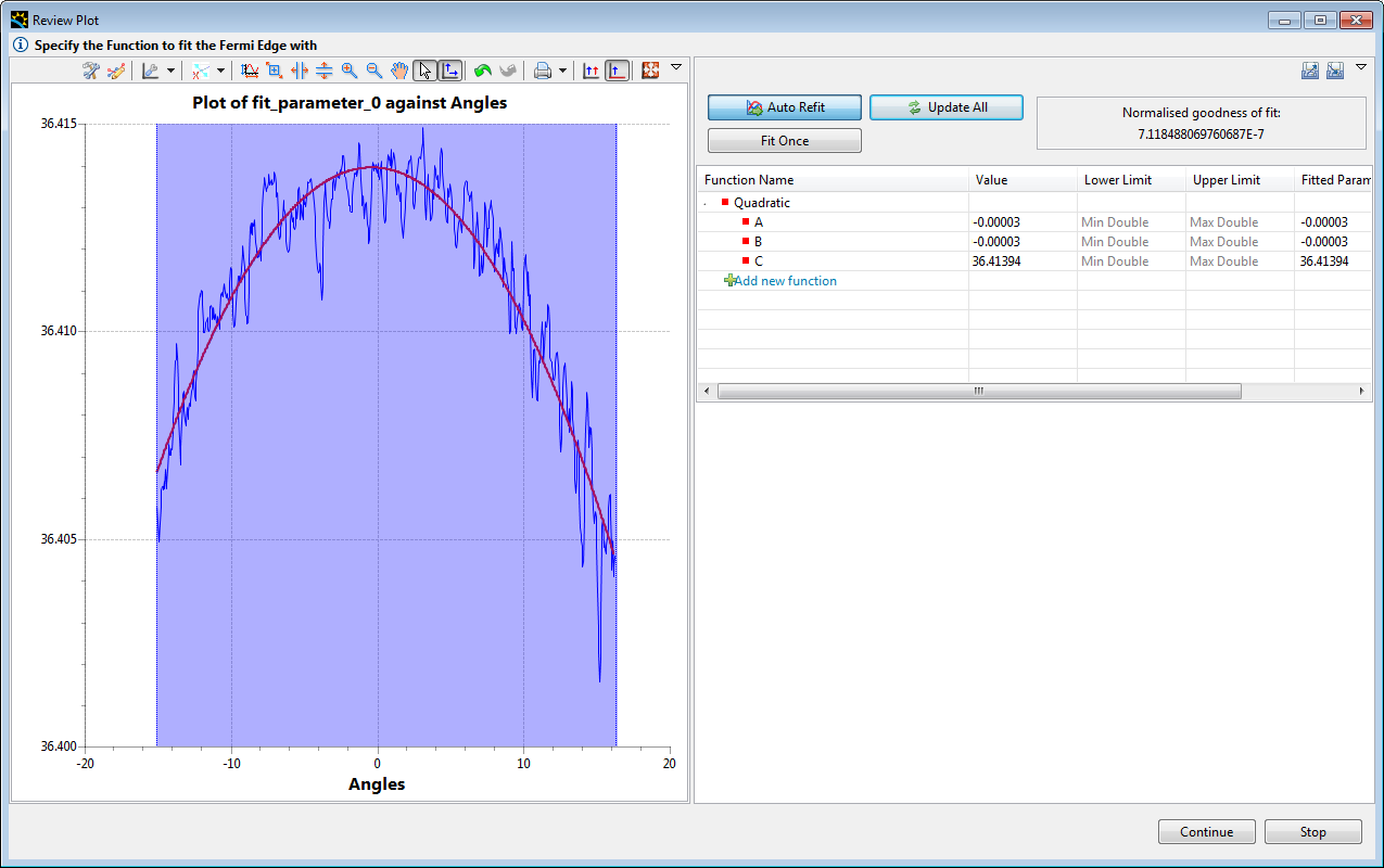
Once you have the function you want selected, use fit once or auto refit to make the selected function fit to the data, make sure you press the Update All button to set the parameters.  Be aware that the smoothed function has 2 parameters, the smoothing one is apparant when you change it, but the tail_proportion parameter is the proportion of each side of the function which is used to extrapolate for data which lies outside the fitted region.

Select where to save the file, and click continue

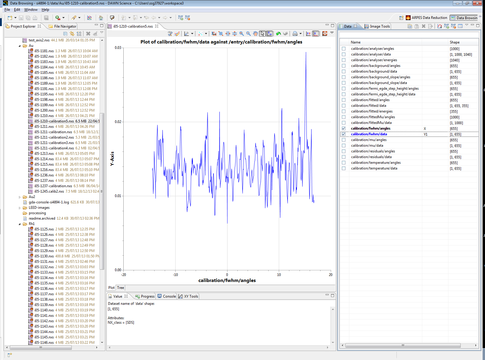
You can now open the calibration if you like to see the reuslts, and check other parameters if useful

Processing a data file

First open the processing perspective, with Window -> Open Perspective

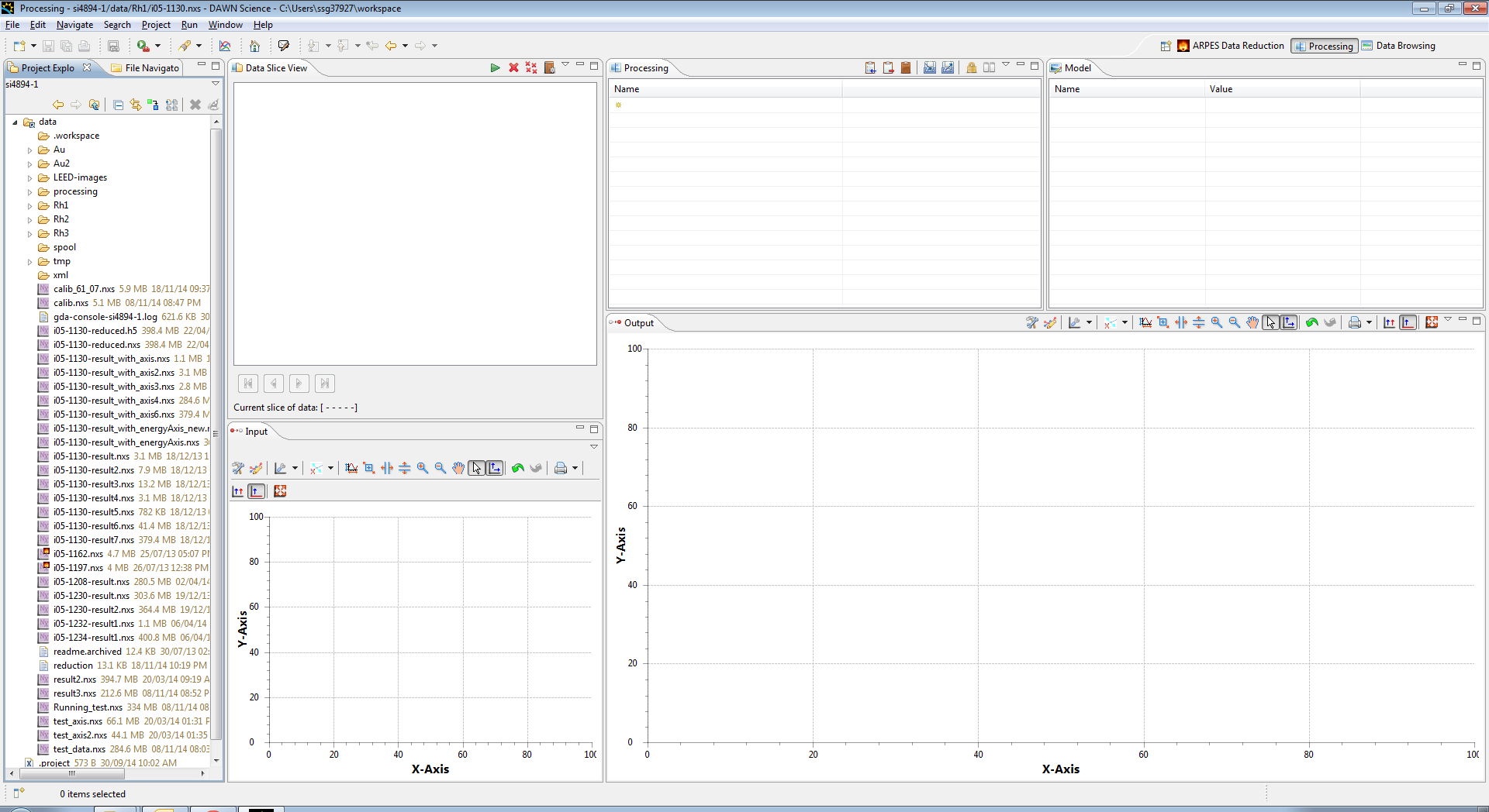
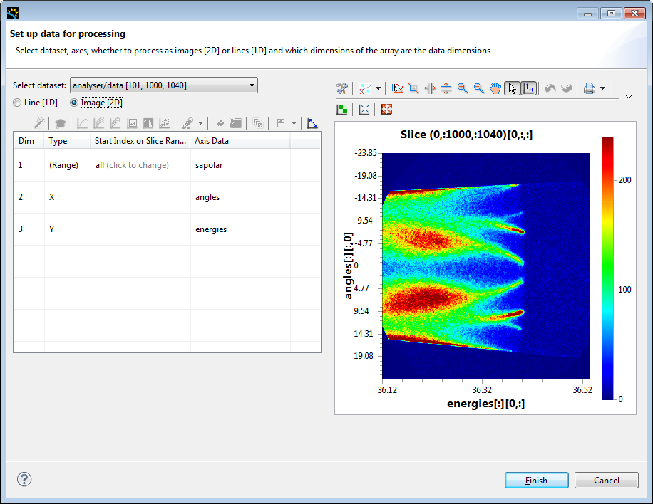
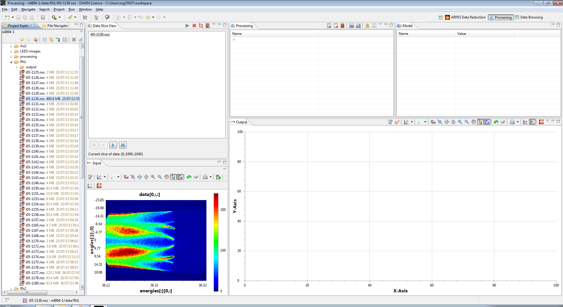
Now select a file you wish to process, this can be done by double clicking on it, or dragging it into the Data Slice View.

When you do this a window will display, asking you to select the appropriate data, With ARPES the default should be correct, so just click Finish.

You should then see the filename appear in the Data Slice view, and a preview image appear in the Input view

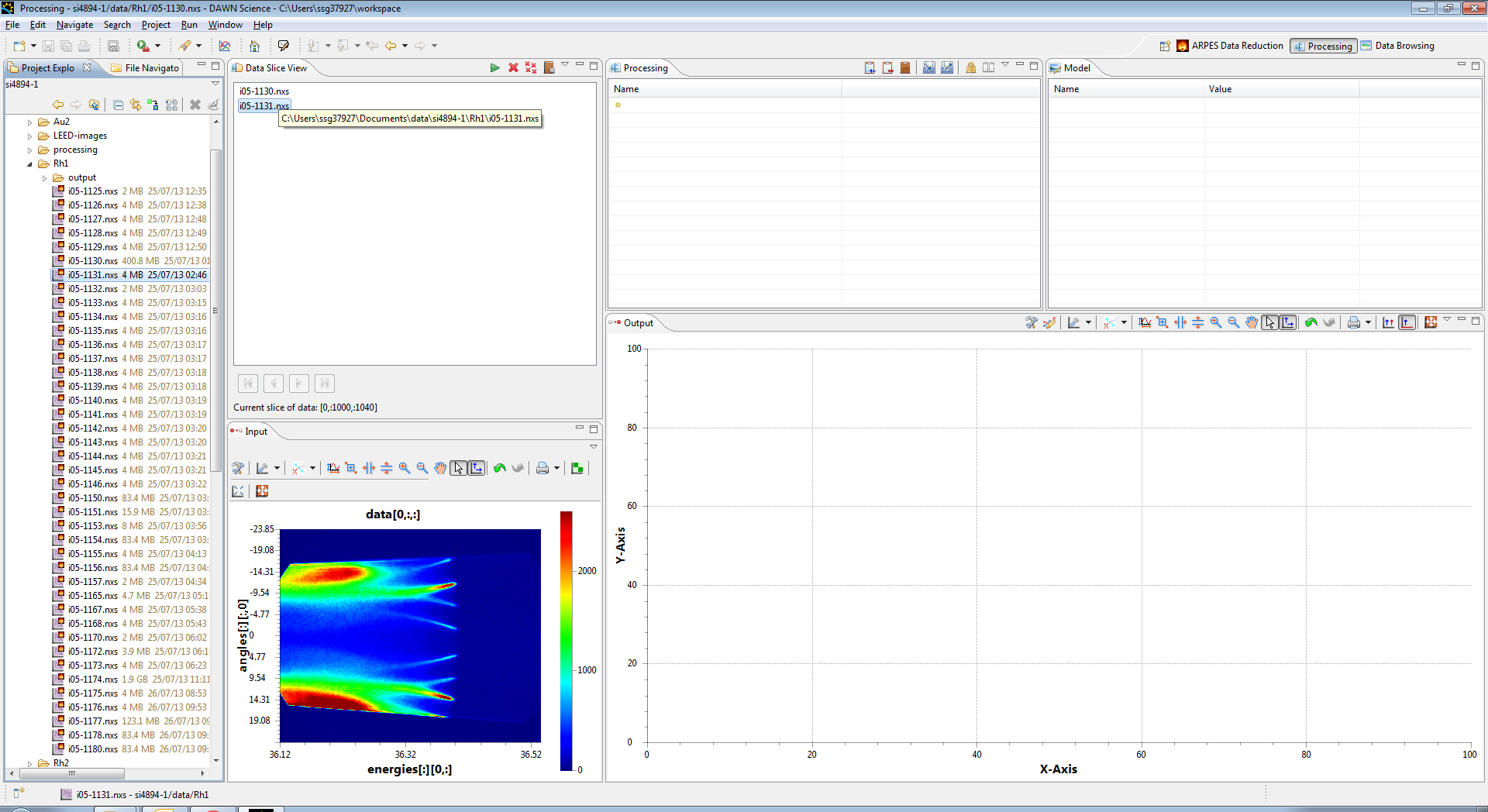
You can add more files by dragging them in, and if they have the same data they will stack up.  you can select which data is in the input window by selecting these files in the Data Slice View, and it is possible to view any slice using the arrows at the bottom of the view

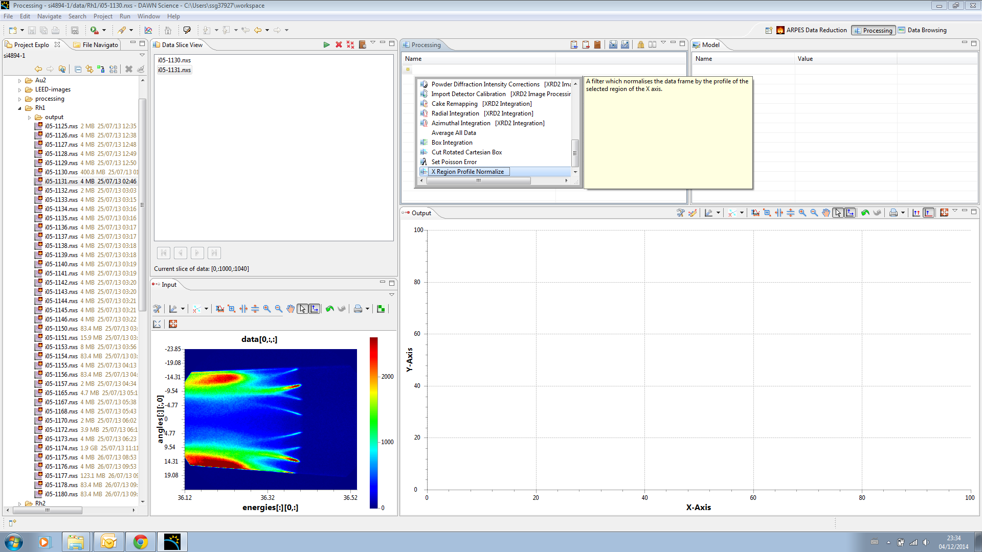
Now we have the input data you can build the processing pipeline.  This may seem a lot of effort but bear with it, as it becomes significantly easier once you have done the initial work.

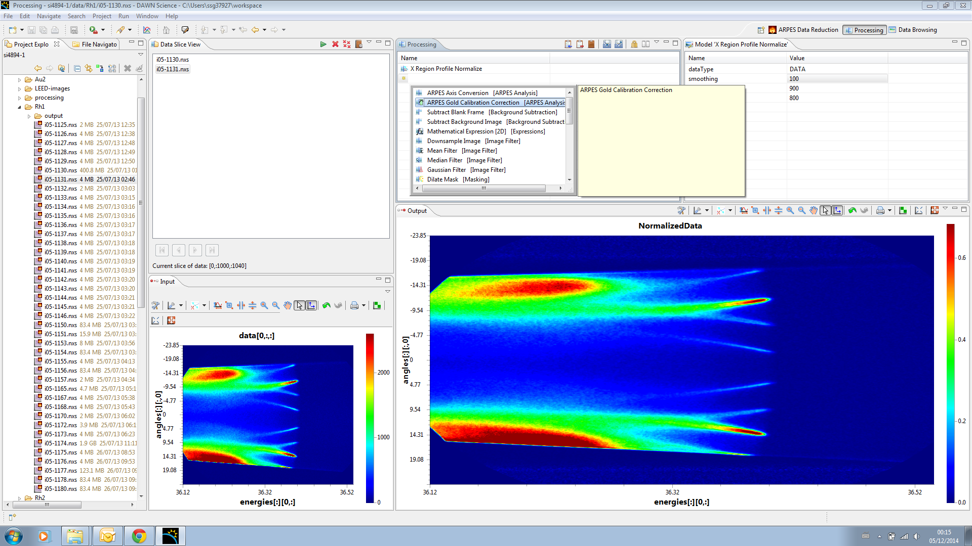
First step is a normalisation against a region of the detector image above the fermi edge.  In the processing view add a new processing element "X Region profile Normalize"

When you do the Output region will populate with the result of the operation we are now applying to the input frame of data.  DON'T PANIC, it looks bad now, but thats just cause the initial parameters are set badly 

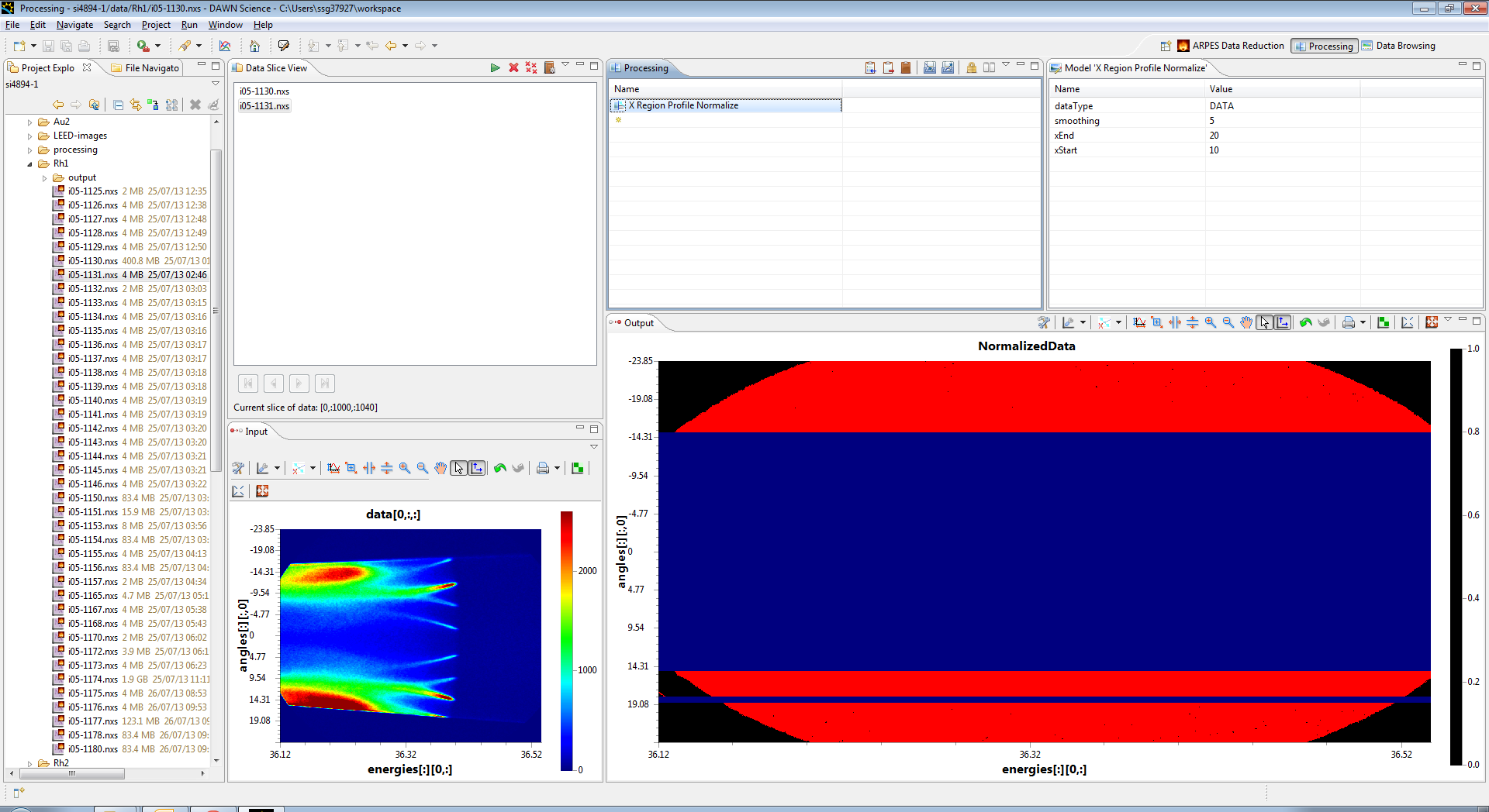
In the top right section, set the xEnd parameter to 900 and the xStart parameter to 800.  This selects the right of the image (above the fermi edge between pixels 800 and 900 in x (Energy)) and then averages it together to form a profile.  The whole image is then divided by this profile, which produces the following normalised output.  You need to click back on the operation in the processing view. 

The result now looks a lot better, but it is still a little streaky, so we can up the smooth value (set to 100) to smooth out the profile before applying it to the frame, which makes the data look a lot better. (Remember to click on the operation again to refresh the data)

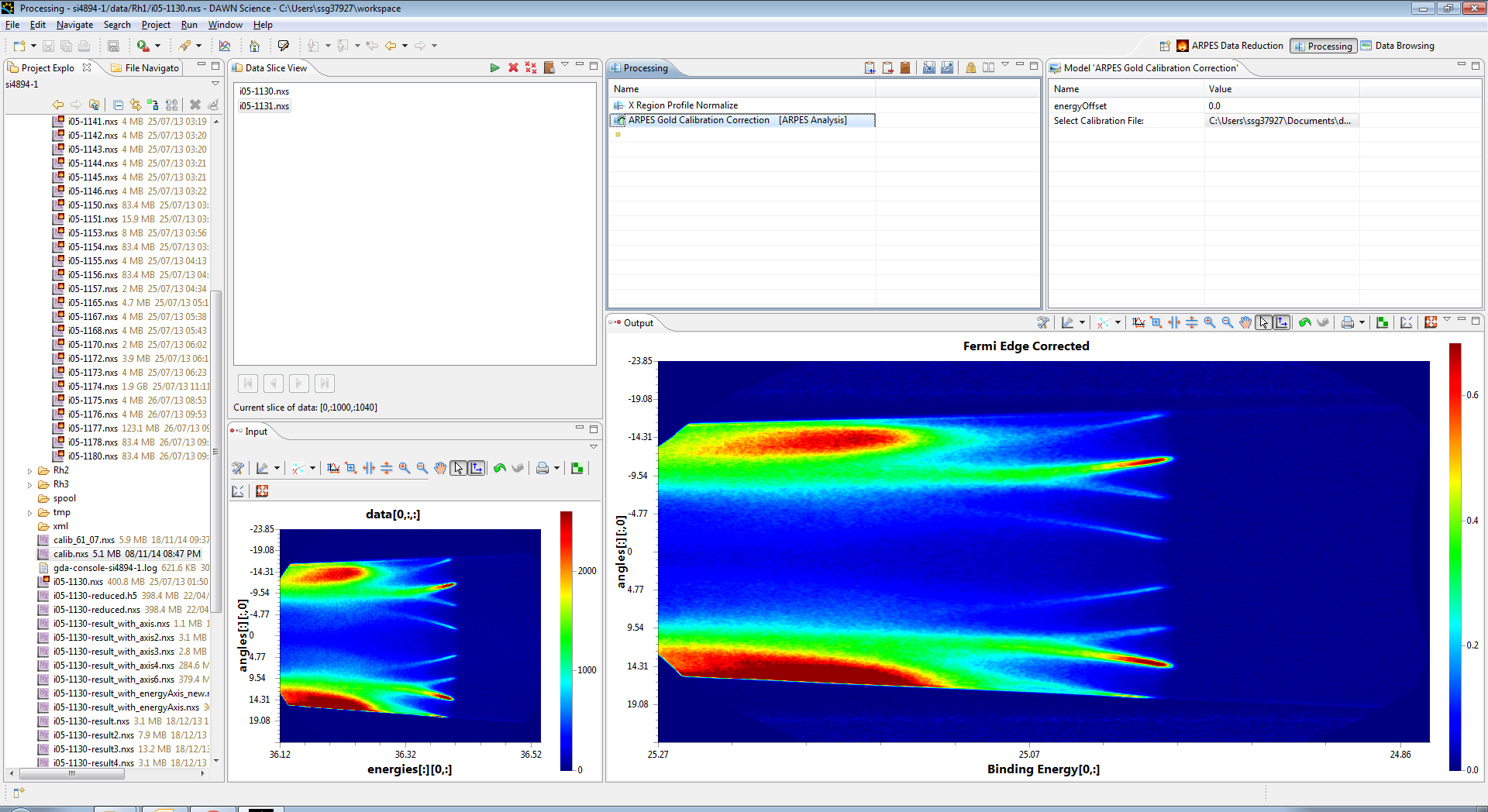
Now the data is intensity normalised, we should correct the gold edge, to do this add the ARPES Gold Calibration operation to the operations list.

This operation needs to have a previously calculated gold calibration file entered as its input, and then click back on the operation to apply the correction, you should see the curve removed from the data.  At this point you can select teh steps in the process in turn to see how they effect the output, as the output only shows the processing down to the selected operation.

The energies are sorted out, but we now need to change the angles to momentum space, to do this we use the ARPES Axis conversion operation, and apply the results, you should see the angles axis turn to Kx.

Although not required, you can now choose to downsample the output, which makes it easier to visualise in some packages, Add the Downsample Image operation to subsample each image.

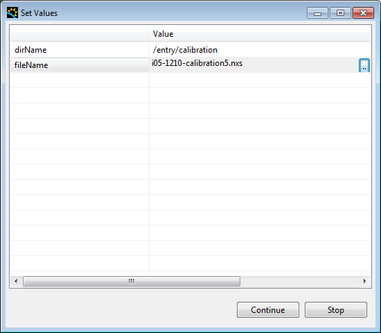
Congratulations, the pipeline is complete, and now you can process all the data in the Data Slice View by clicking the play icon at the top of the view, which will bring up the following dialog to fill in where you want the data to be outputted.

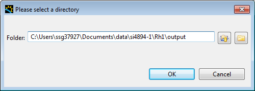
Click Ok and the processing will start.

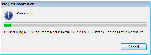
The processing is complete, but the pipeline is saved in the output file, if you want to reload a pipeline, simply drag an output file into the Processing view, and the operation list will be loaded.

You can also export the process list using the export option at the top of the processing view.

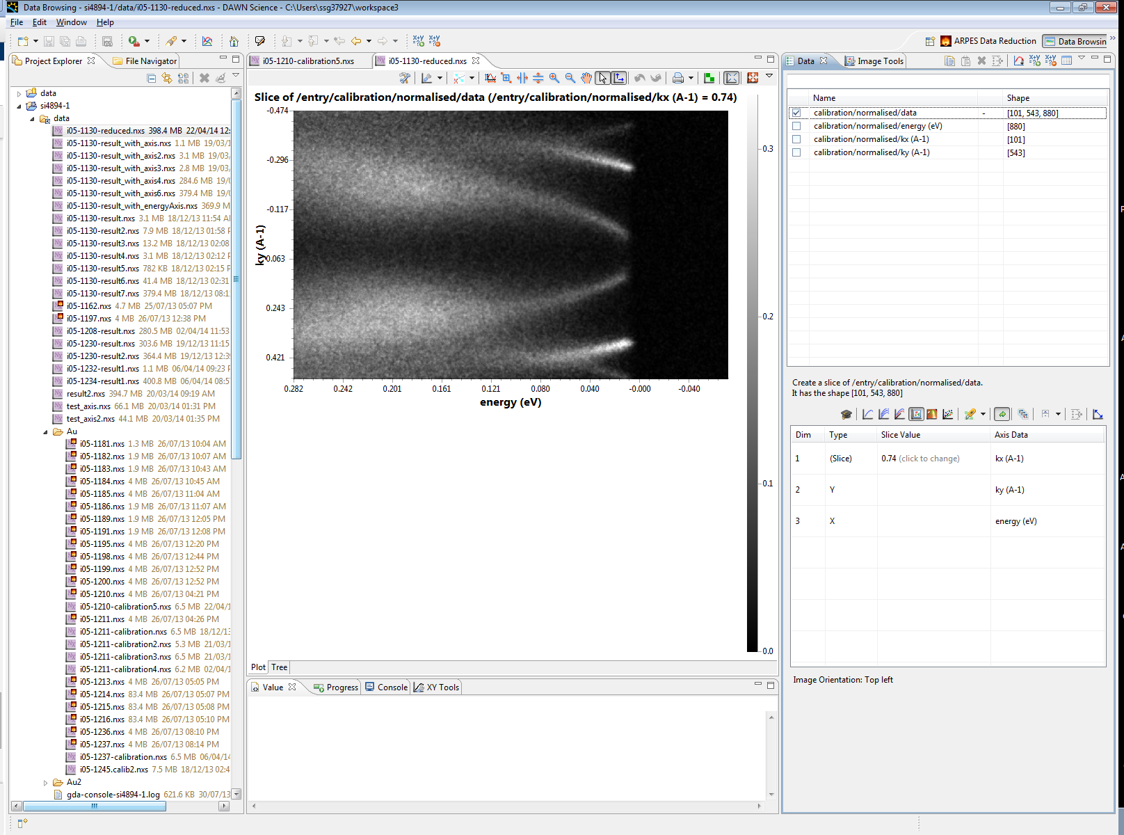
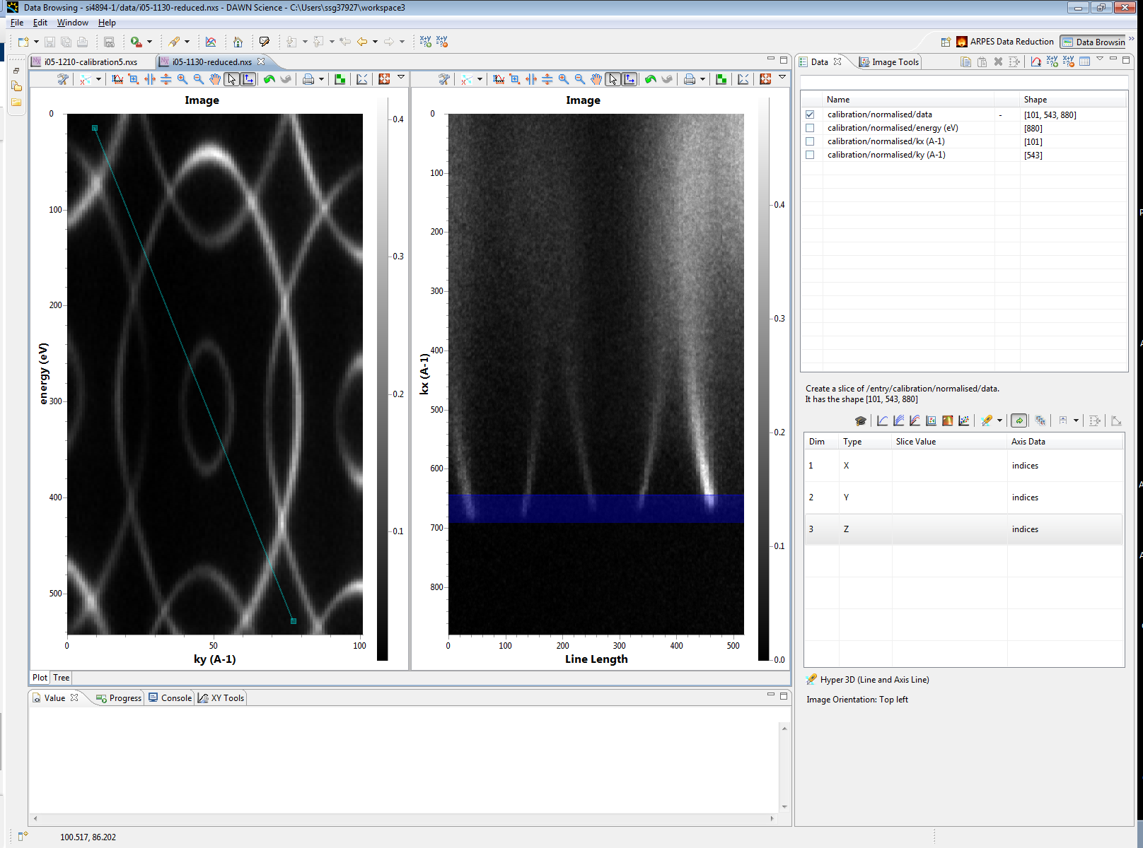
Once the processing is completed, the results can then be visualised using the data browsing perspective