Quick start to guide to using the DAWN mapping perspective to visualise data from I05-1

Viewing Map Data

1.  Start DAWN (module load dawn on a diamond linux workstation or download from dawnsci.org)
2. Open the Mapping perspective (Window/Perspective/Open Perspective/Other... then select mapping from the list)
   
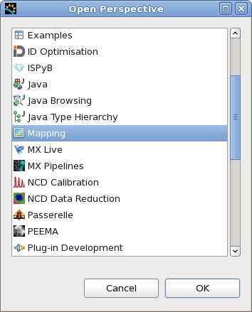
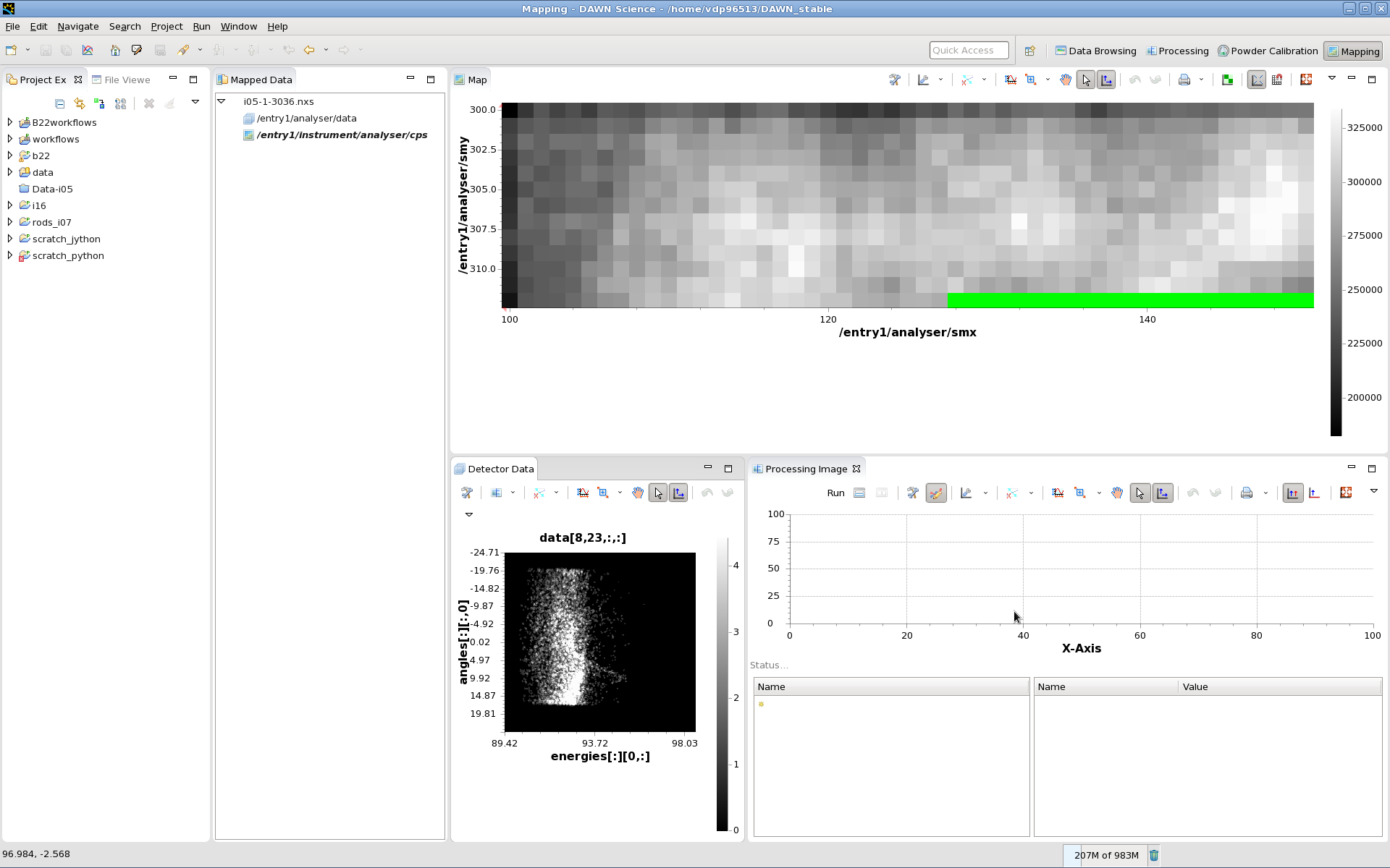
3. Mapping perspective should now be shown
   
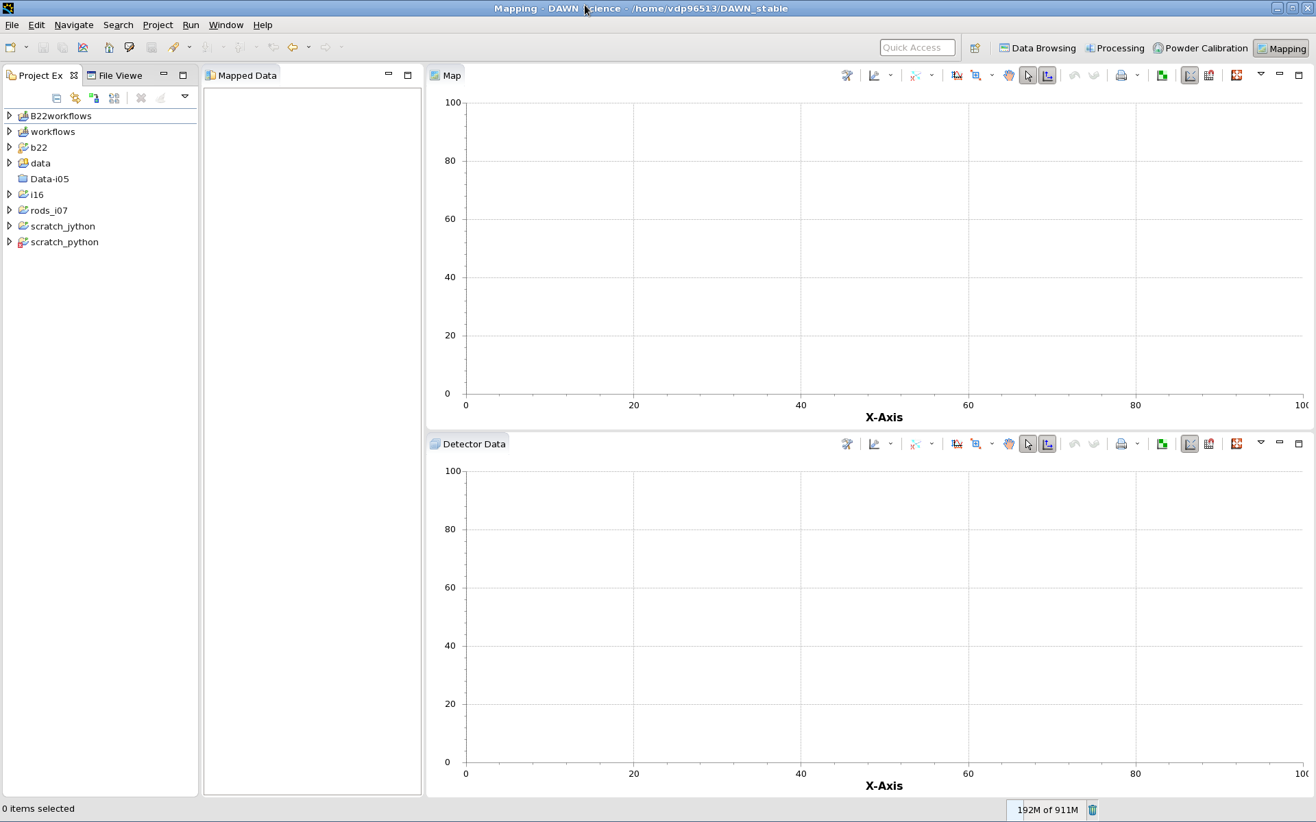
4. Open a mapping scan (File, Open Map File... or drag from the operating system file explorer into the Mapped Data table)
5. The file should automatically load the Counts Per Second map, clicking on this map should show the analyser image associated with the pixel of the CPS map clicked.
   
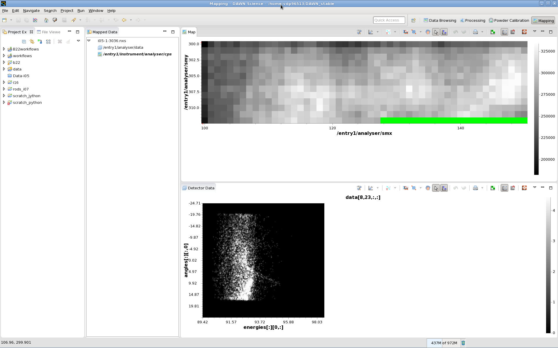
6. Multiple maps covering similar areas of the sample can be loaded for viewing at the same time.

Basic Processing of Map Data

1.  On the plot showing the detector image (Which changes when you click on the map, in the Detector Data tab), open the tool menu (wrench icon with axis) and select Processing Image
   
   
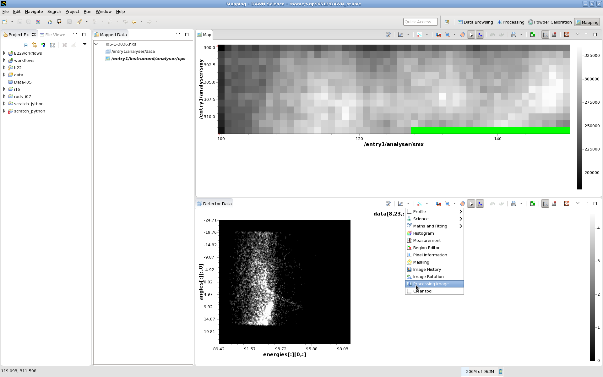
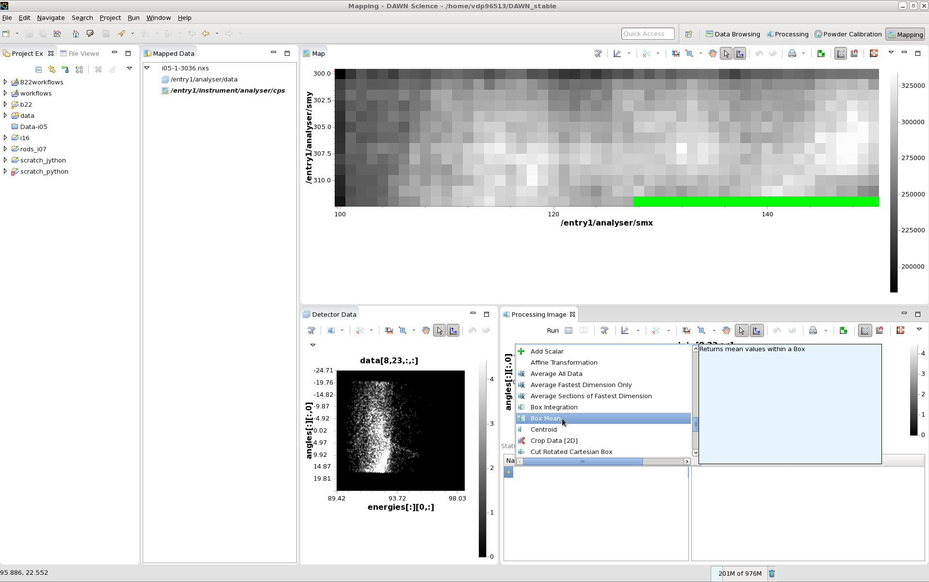
2. The Processing Image tool will open (probably behind the Detector Data tab, drag the Processing Image tab to be next to the Detector Data tab as shown below)
   
3. This tool allows you to generate new maps by averaging data in a specific region, or from the difference between two regions, the data can also be integrated across all angles to 1D
4. Click on the small yellow start to see the list of all processing steps and select Box Mean
   
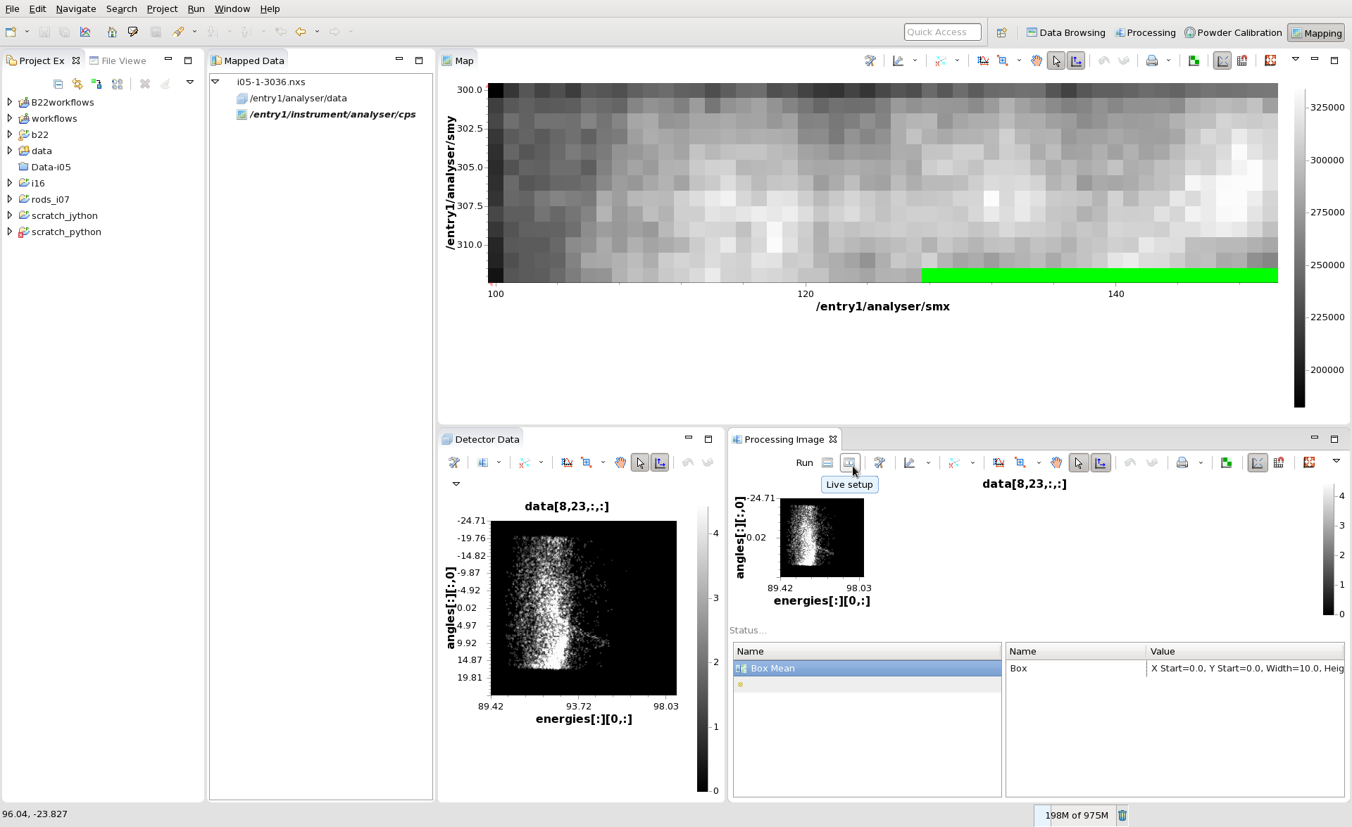
5. Select the Box Mean entry and press the live setup button
   
6. In the dialog that appears, move the box to cover the region to be averaged and press ok
   
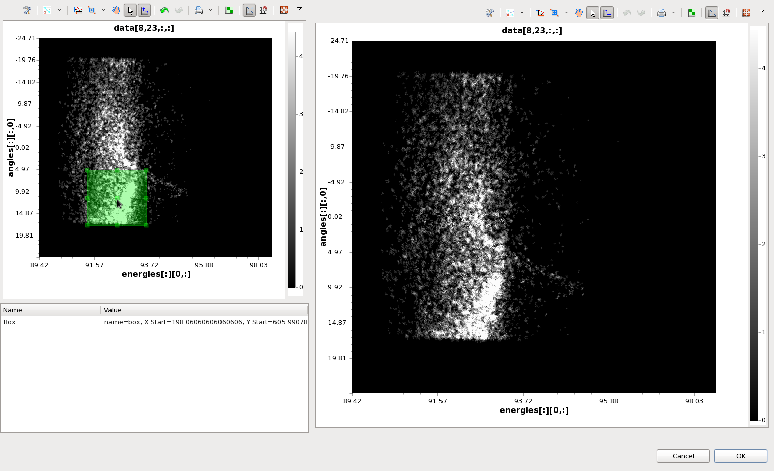
7. Many Box Mean ( or Two Box Mean Difference...) steps can be added with different boxes by repeating the last 3 steps. Processing steps can be remove by pressing delete.
8. Click the yellow star again and this time add Image Integration (when you click the star you should be able to start typing image to filter down the options)
9. The Processing Image tool window should now show a 1D plot against energies
10. Pressing the "Run" button (near the live setup button) will cause this processing to be done to all images (select a suitable location for the processed data to be saved, the data processing may take a long time)
    
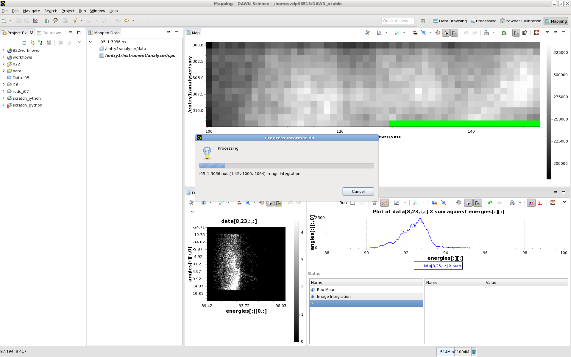
11. When the processing has finished, the processed data should be automatically loaded, with the new map being displayed. Clicking on the new map should now show the integrated, 1D data.
12. 
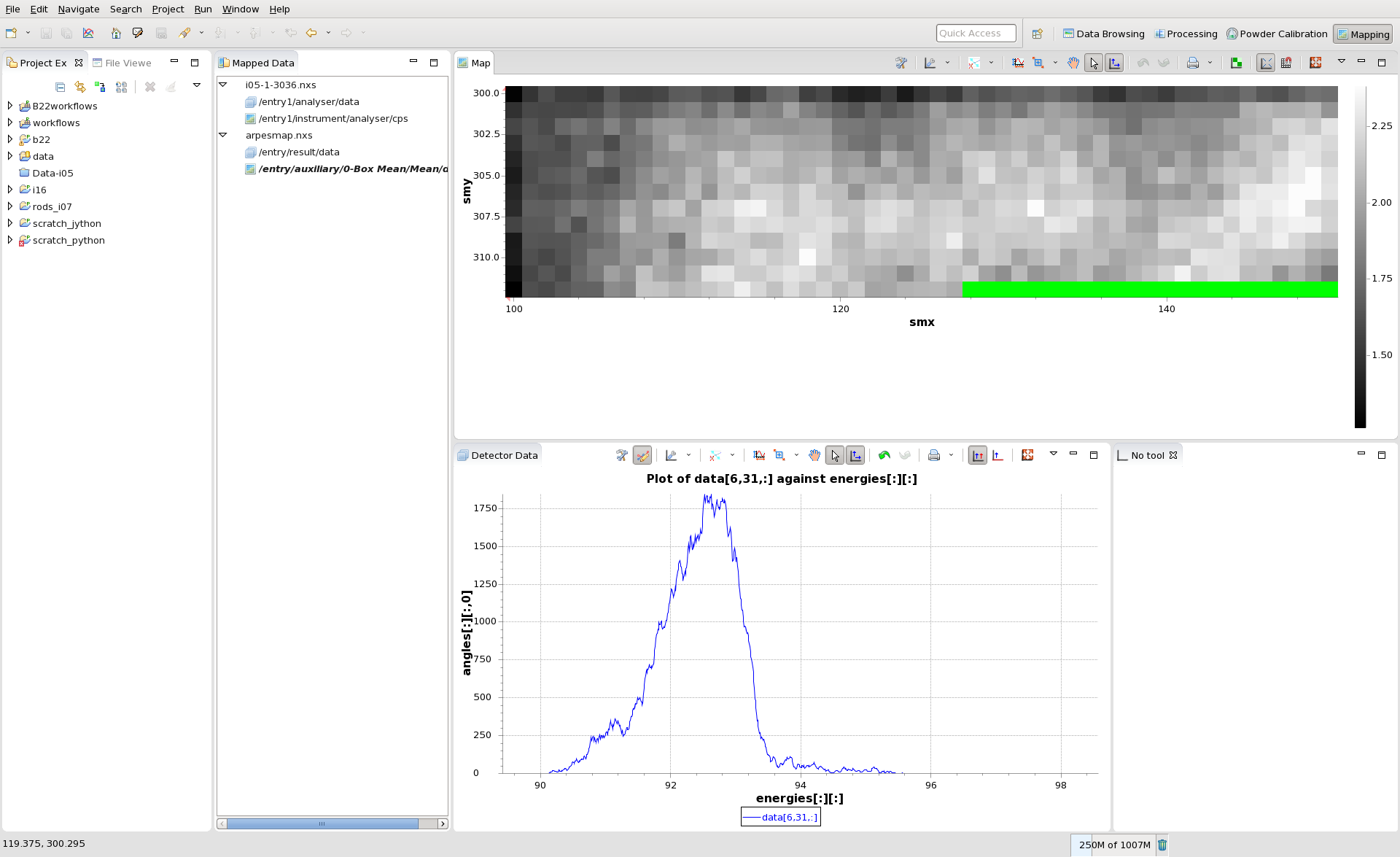
13. You can switch back to looking at the original map and 2D detector image by double clicking the cps entry in the Mapped Data table
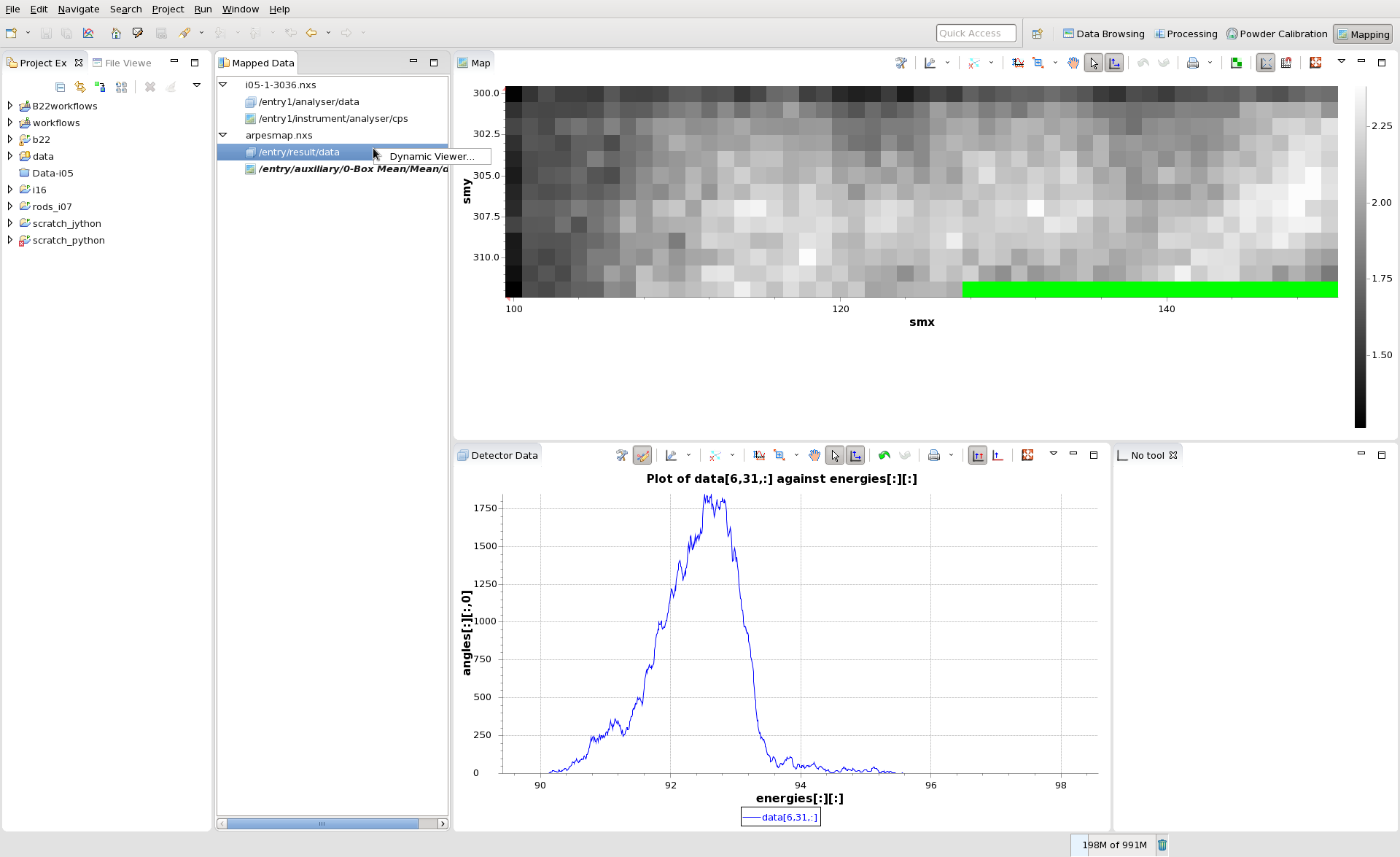
14. The integrated data can be interrogated dynamically using the dynamic viewer (not possible for the raw detector images)
15. Right click on the /entry/result/data entry in the processed file in the Mapped Data table and select Dynamic Viewer
16. 
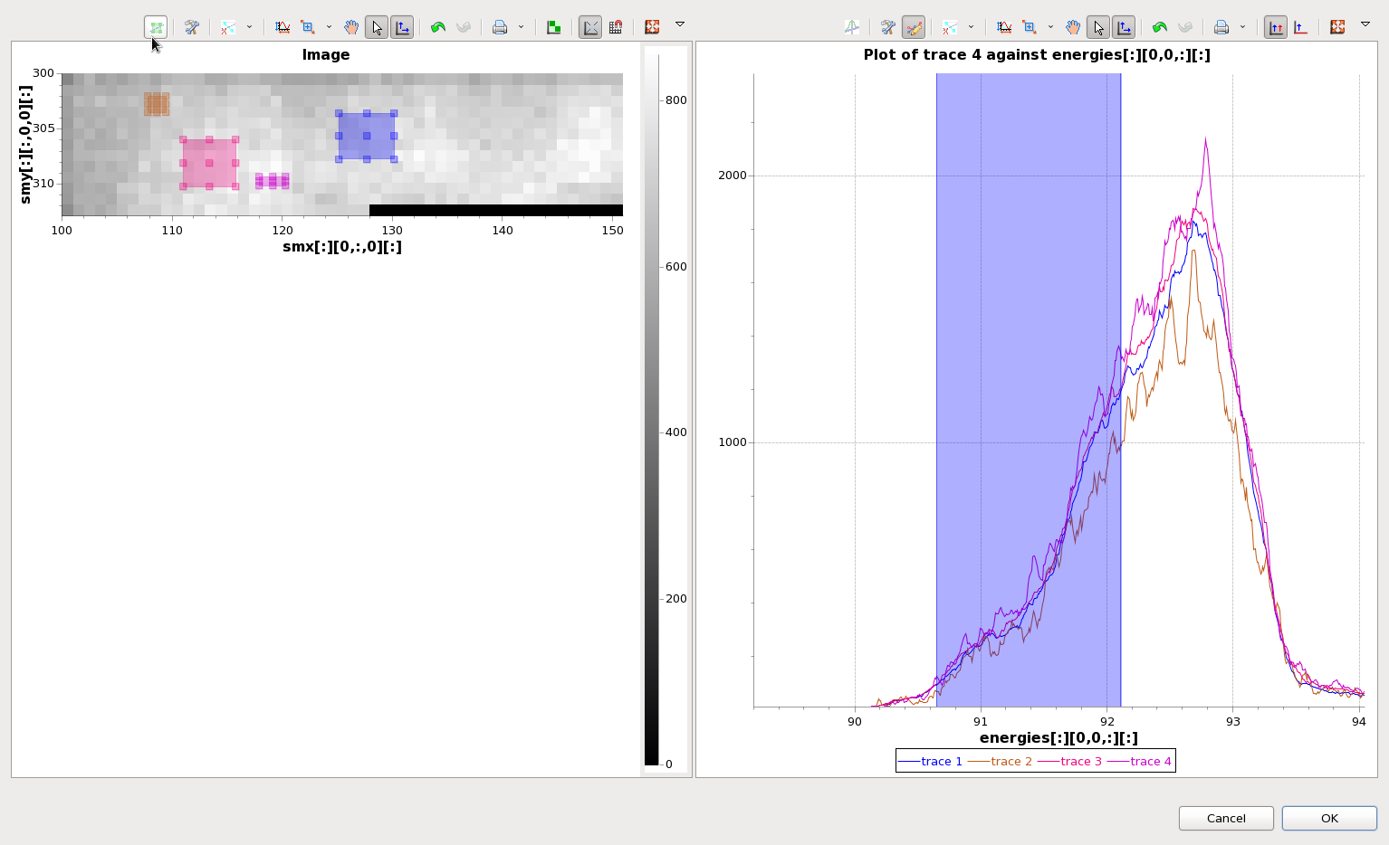
17. The Dynamic View dialog should open, showing a map on the left and a spectrum on the right.
18. The box on the left plot defines the region to be averaged to produce the spectrum
19. The region on the right plot defines the region of the spectrum to be integrated to make the map
20. More box regions can be added to the map by clicking the Create new profile button on the plot tool bar (far left)
    
21. The average spectra can be exported to text using the Export data to tif/dat action on the plot tool bar (export options drop down, next to the printer icon.