Mapping Perspective
Introduction
The mapping perspective is designed to view NeXus files from a specific type of experiment; one in which the sample was scanned while measurements were being taken.
For these experiments, files often contain two different type of datasets; Maps - a single value per measurement point, which when displayed reflect the real space structure of the sample, and Data Blocks - the raw or reduced detector data taken at each measurement point - usually a 3D or 4D dataset.
The Mapping perspective allows multiple Maps, from different files, at different spatial locations on the sample, and with different resolutions to be viewed at the same time. The underlying raw or reduced data can be investigated by interacting with the displayed Maps.
In this user guide a Infrared Imaging measurement on cancer cells is used as a demonstration. The four files used (one white light microscope image in a NeXus file, two IR spectra imaging data files and a jpeg image file) can be downloaded using these links:
https://alfred.diamond.ac.uk/DawnExampleData/microscope.nxs
https://alfred.diamond.ac.uk/DawnExampleData/ftir1.nxs
https://alfred.diamond.ac.uk/DawnExampleData/ftir2.nxs
https://alfred.diamond.ac.uk/DawnExampleData/image.jpg
Loading and Displaying Data
Switch to the Mapping Perspective.
Data can be loaded simply by using File/Open (as shown in the Quick Start Guide) or by one of the other methods (as shown in the Opening Files Guide #TODO make this).
Load the file ftir1.nxs into the mapping perspective. A tree representing the files should appear in the Mapped Data view. The three nodes of the tree represent the Data Block (in this case the IR absorbance spectrum - one spectrum per scan point) and two Maps (map1 and map2).
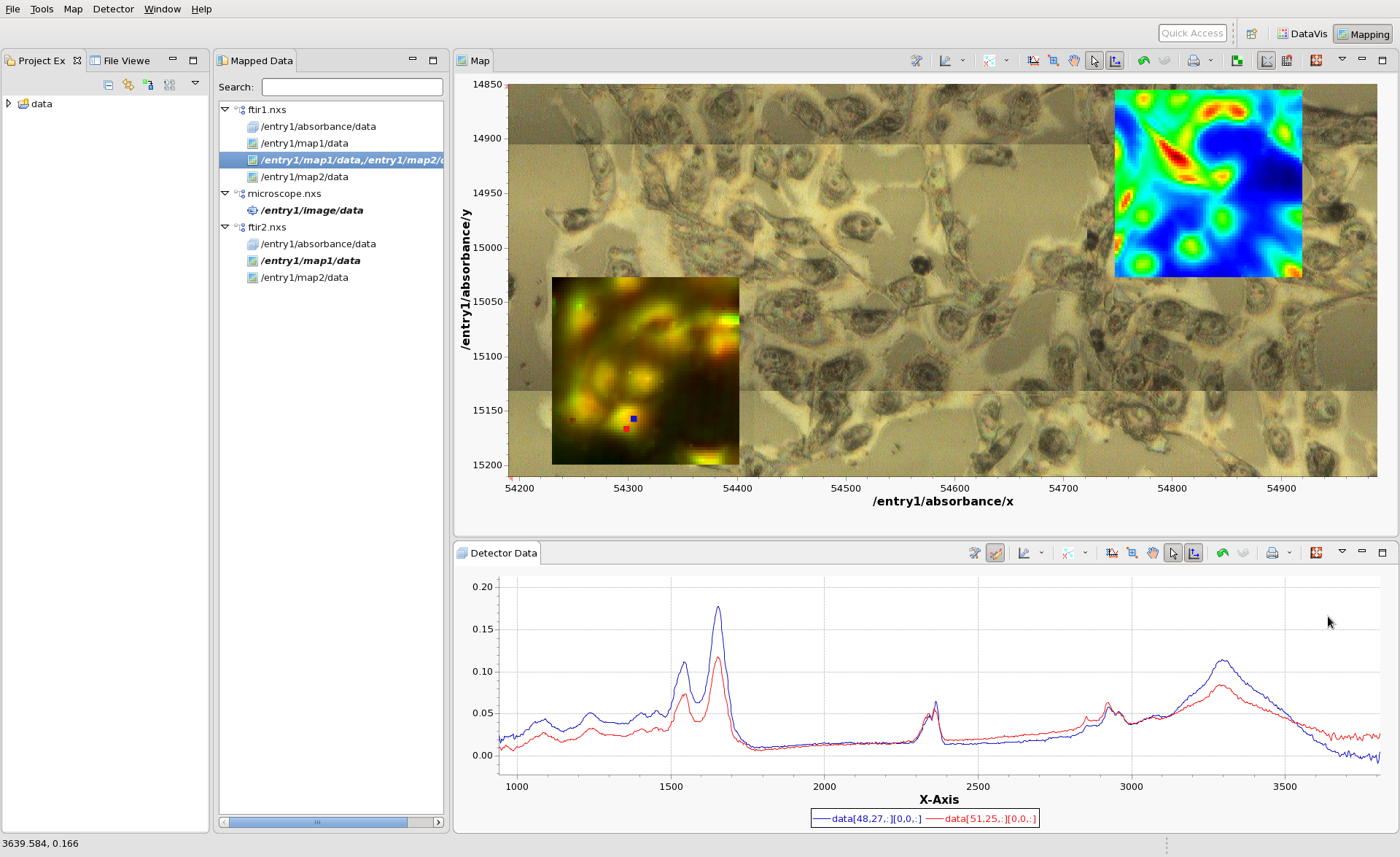
Double click on map1, to display in in the Map view. An image should appear, with x and y values as its axes. Click anywhere on the image to see the IR spectrum from that pixel. Hopefully by now your mapping perspective looks something like this:
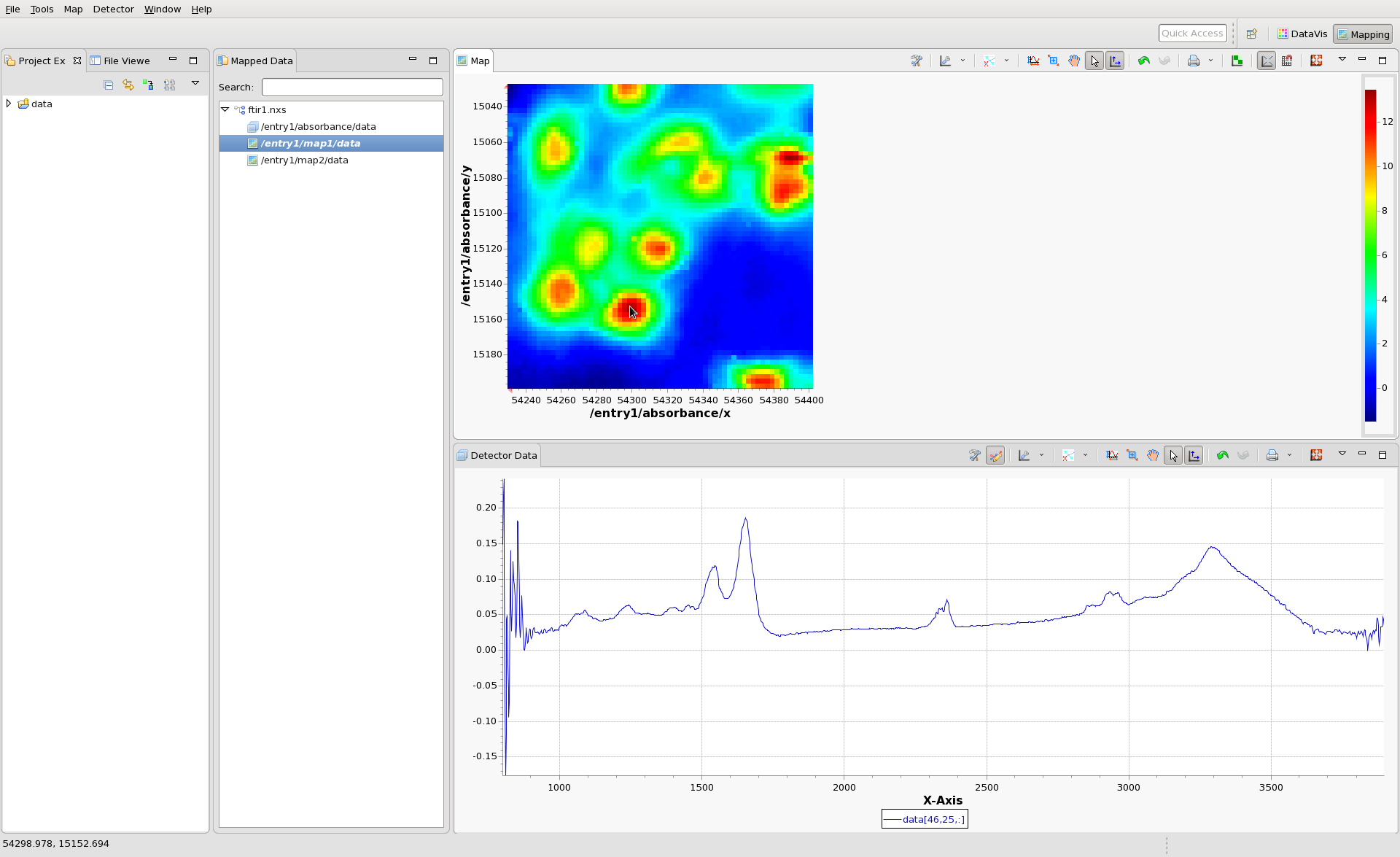
(The colormap and contrast/brightness of the map can be adjusted by following the Colormap Guide #TODO make this). Holding shift and clicking on the will display multiple lines on the Detector Data plot and a marker on the Map plot showing where the data came from. If the scan you are viewing collected images, rather than spectra at each point, clicking on the Map would show an Image in the Detector Data Plot. For images shift-clicking allows a montage image to be created.
Double-clicking on the map2 entry will unplot map1 and display map2 instead. The mapping perspective will still show the underlying data on clicking whether map1 or map2 is shown.
Displaying Data From Multiple Files
The Mapping perspective allows simultaneous viewing of multiples files, acquired using different experimental techniques as long as they have the same spatial axes on the sample.
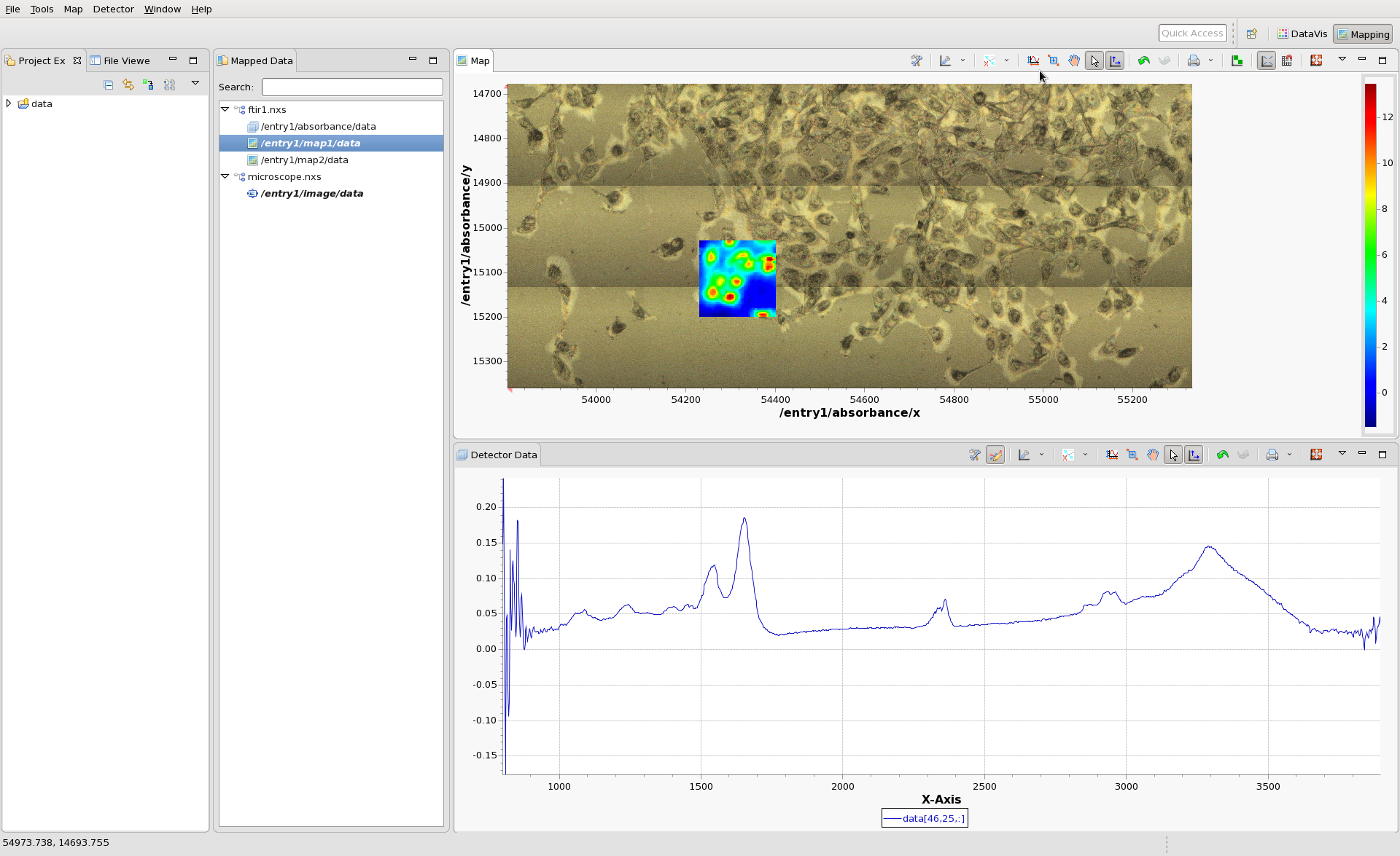
Load the microscope file, microscope.nxs and double-click on the image node in its tree. The Mapping perspective should now show the IR data from ftir1.nxs on top of a microscope image of the cell sample from microscope.nxs
Now also load ftir2.nxs and select map1 to plot. Try using shift-clicking to overlay the IR spectra from pixels in ftir1.nxs and ftir2.nxs.
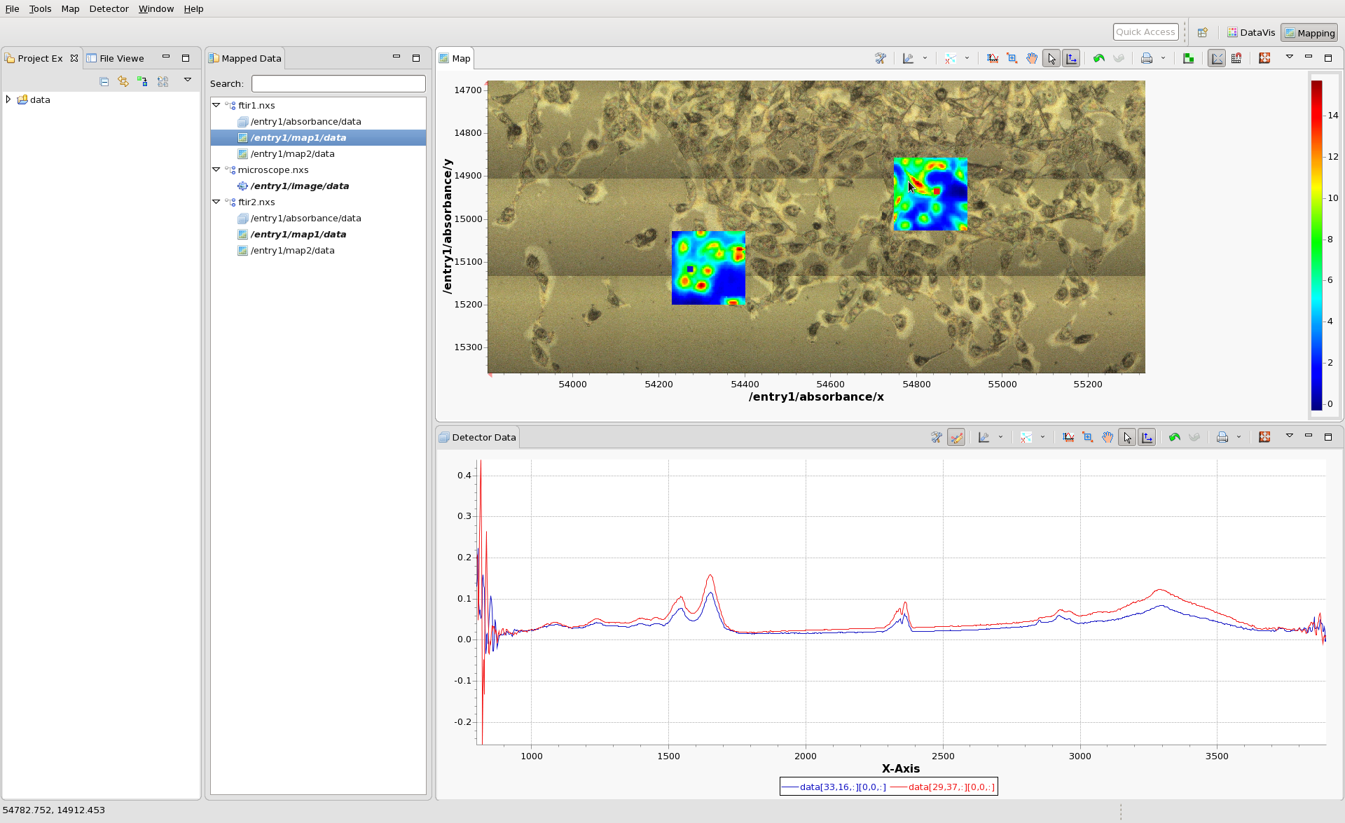
Using the tree structure in the Mapped Data View is should be possible to display combinations any combination of images from the 3 files (except for images that perfectly overlap - map1 and map2 from ftir1 cannot be viewed at the same time).
Further Viewing Options
Transparency
When two images overlap each other (in this example the IR image and the microscope image), it is useful to be able to adjust the transparency of the top image to see how well it matches features in the image below.
Make sure both the microscope image and map1 from ftir.nxs are displayed, select map1 in the tree and right-click on it. In the menu that appears select Properties...
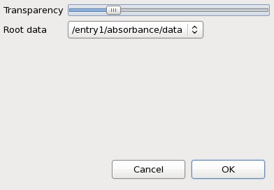
The transparency of map1 can be adjusted using the slider in the dialog.
![]()
Comparison Viewer
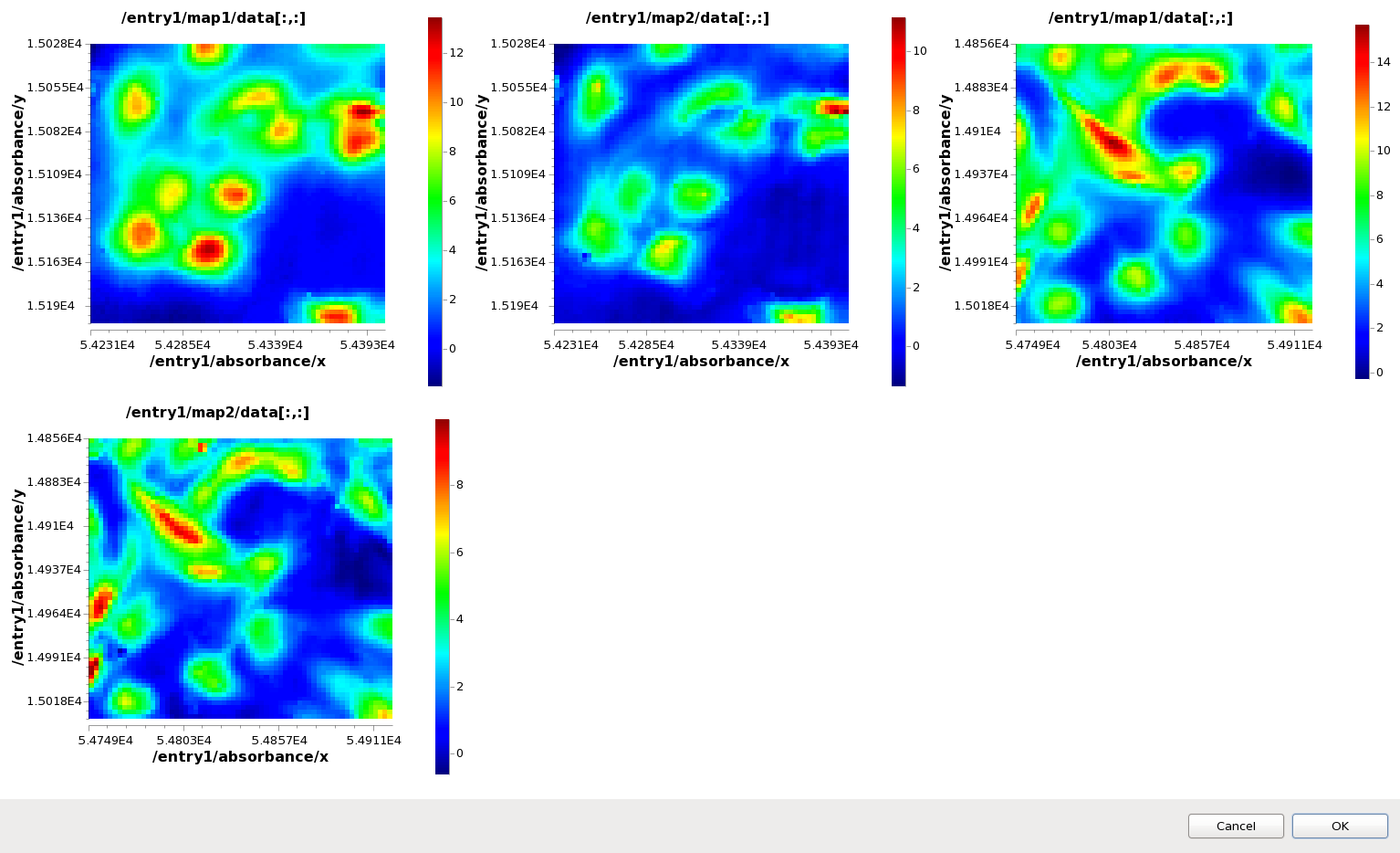
Use ctrl-click to select all four maps in the Mapped Data view tree (map1 and map2 from ftir1.nxs and ftir2.nxs). Right-click on one of the maps and select Comparison Viewer...
The Dialog that appears shows all the maps plotted at the same time in different subplots, and is a quick way to look at multiple maps from multiple files without loading them into the main Map plot.
RGB Mixer
The RGB mixer allows maps to be used as Red, Blue and Green channels in a "fluorescence-style" blended false colour image.
This time just select map1 and map2 from ftir1.nxs, right-click and select RGB Mixer...
In the dialog that appears select map1 for the red channel and map2 for the green channel. Use the double-arrow slider to adjust the min-max color mapping of the red channel.
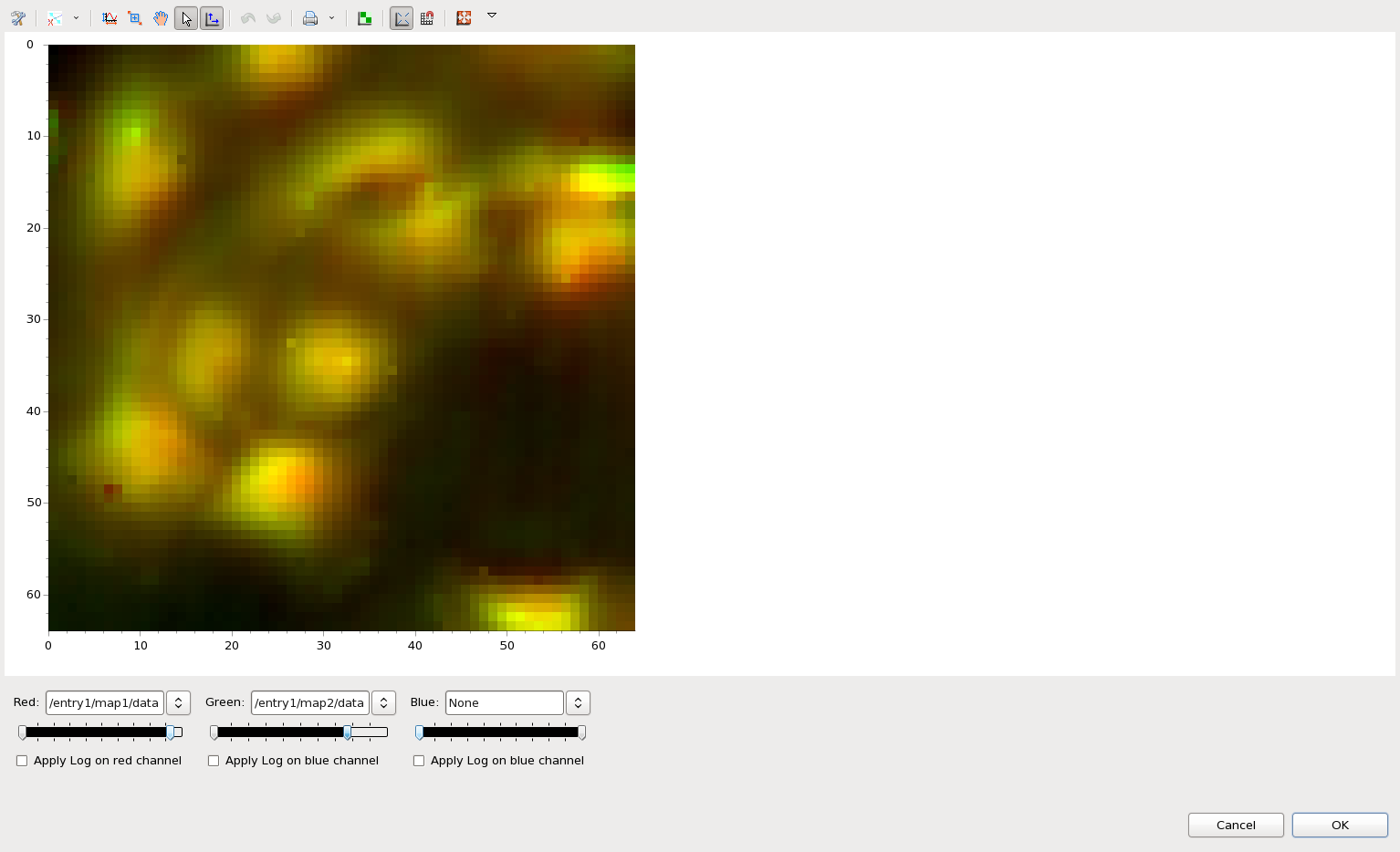
Clicking OK adds an additional map to the ftir1.nxs tree, which is this new combined image. It can be added to the main Map plot by double-clicking, in the same way as the other maps.
Files Containing Multiple Data Blocks
In the supplied example data there has only been one data block that the maps relate to - the FTIR absorbance spectrum. It is very common for their to be more than one data block associated with a map. For example, a map generated using a 2D diffraction detector might want to display the raw detector image, or the reduced 1D powder diffraction pattern. If a file contains multiple possible parent data blocks for the maps it is possible to select which block should be seen when clicking on a map by using the Root data drop-down box on the Properties dialog.
Registering an Image File
It is possible to read in a standard image file (jpg for example) into the Mapping perspective and use one of the maps to register the image into the stage co-ordinate system. This allows sample images from different techniques (light microscopy, electron microscopy etc) to be shown as a background image in the Map plot.
Unplot all the data in the mapping perspective then plot map1 from ftir1. Using File/Open... load the file image.jpg. The Image registration dialog will appear.
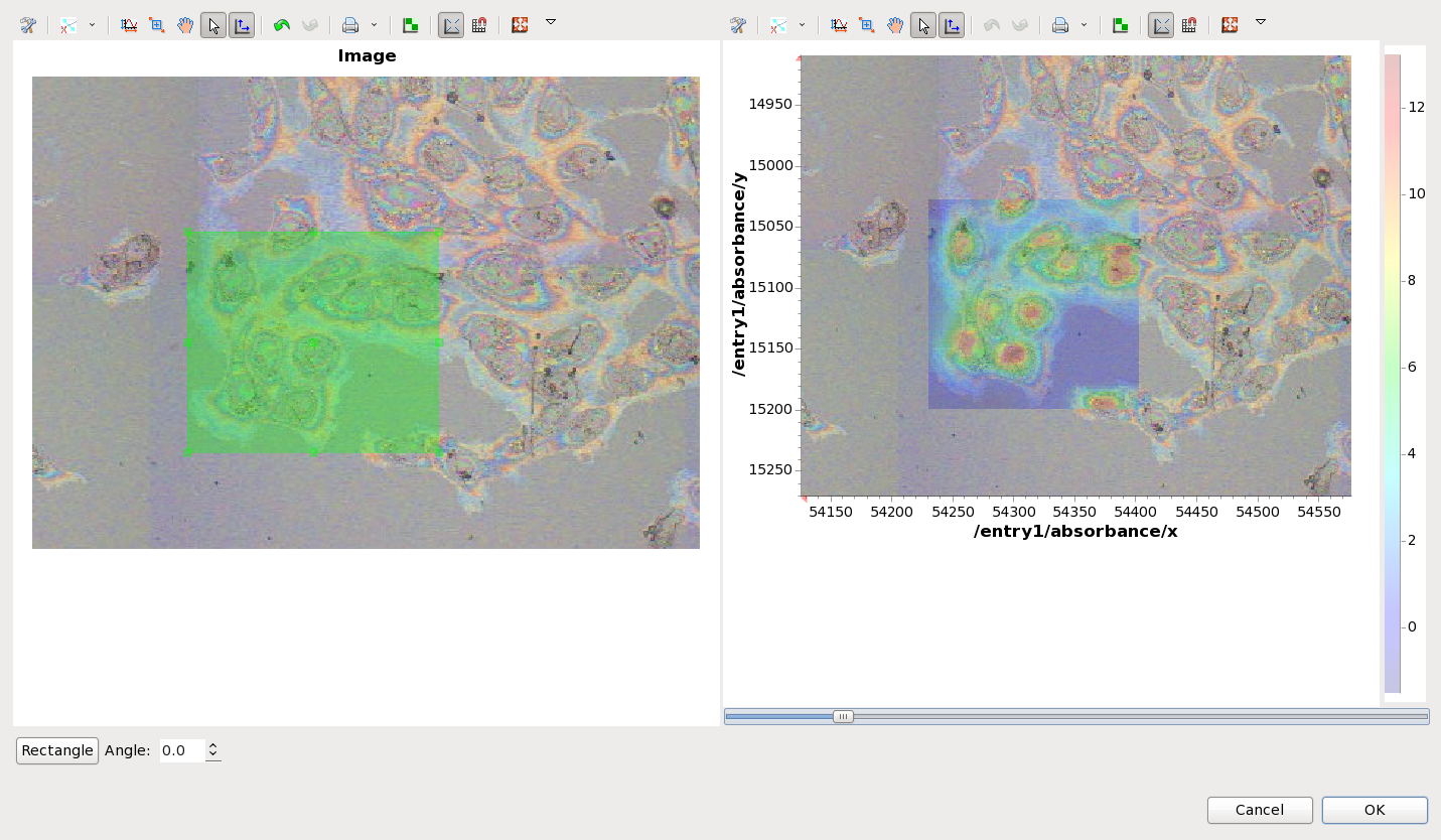
By aligning the green box on the image that was just loaded to the location of the map it is possible to register the image into the map co-ordinate system. The slider below the plot on the right can be used to change the transparency of the map, making the alignment easier. If the input image is rotated with respect to the map it is possible to change the rotation angle of the image by using the spinner at the bottom of the dialog. Once alignment is complete, pressing the OK button adds this new file to the list in the Mapped Data view, where it behaves the identically to the microscope image loaded from the NeXus file earlier.
It is possible to save this registered image into a NeXus file, complete with the co-ordinates, allowing it to be re-loaded at a later date without having to redo the registration. On the Registered image entry in the Mapped Data view, right-click and select Save Image... to chose where to save the NeXus file.
Appendix
File Requirements
For DAWN to recognize a file as being from a mapped data collection it needs to have a specific structure:
- It should be a NeXus file using post-2014 tagging in the NXData groups (i.e. @signal ="dataset_name", @axes = [stagey,stagex,.,.])
- There should be at least 1 NXdata group, and it should contain at least two axes
- These axes can either be associated with separate dimensions of the data block (i.e. a 10x5 scan may have a y axis of 10 and an x of 5), or the same dimension (data from a spiral scan for example that is stored as a flat list).
- If there is more than 1NXdata group, the lowest rank signal dataset defines the maps, any higher dimension datasets are assumed to be Data Blocks (raw detector data, processed arrays per point, etc).
- RGB image datasets should have interpretation tags on the dataset to be recognised correctly.