DataVis Perspective
The DataVis perspective is intended to eventually be a replacement for the DataBrowsing, DExplore and Trace perspectives, with all the functionality they include (and more) in one place.
It is still very much a work in progress with the usability and feature being tested and prioritised by the scientists here at Diamond.
For a really quick intro try the cheat sheet.
Lets get started...
From an open DAWN, the easiest way to access DataVis is by typing DataVis in the Quick Access box and pressing Enter.
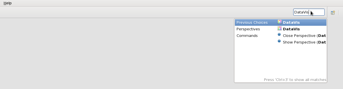
You should see the user interface change to something that looks like this:
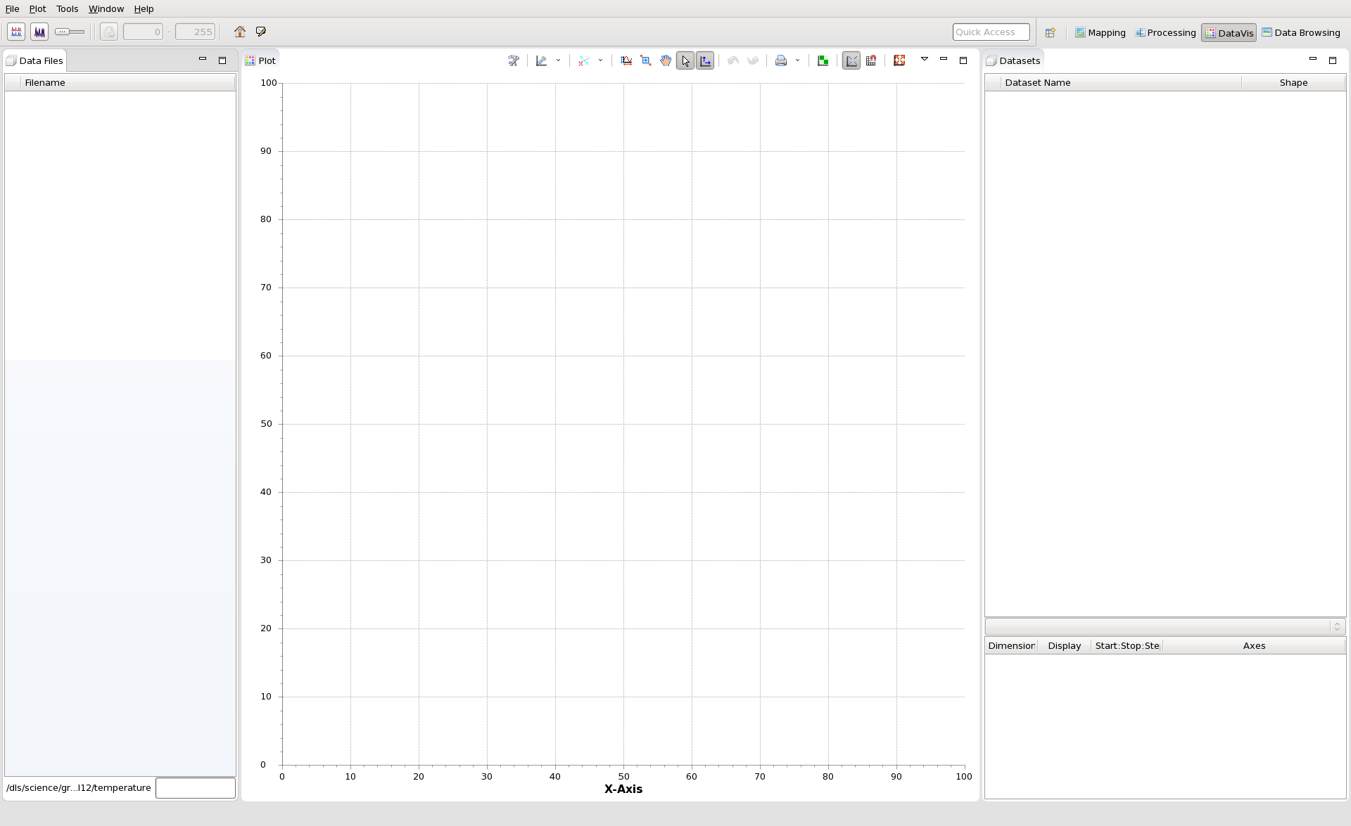
One of the aims of the DataVis perspective is to have a clean, simple user interface. At the moment, DataVis doesn't use the Project Explorer or File Navigator found in other perspectives.
Loading Data
To load data into the DataVis perspective either use the File, Open File... menu, or drag and drop a file into the Data Files View.
As well as Open File..., the File menu contains some other convenient routes to load data.
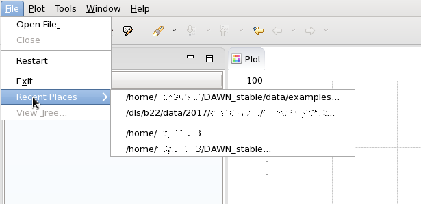
The Recent Places option remembers the last 5 folders data was loaded from, as well as containing a link to the home directory and the DAWN workspace (just in case you want to access some data from the project explorer). Files can also be loaded using the Quick File Widget.
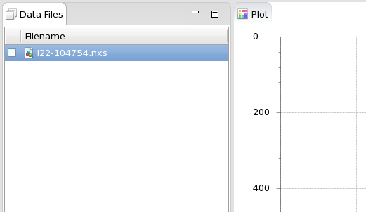
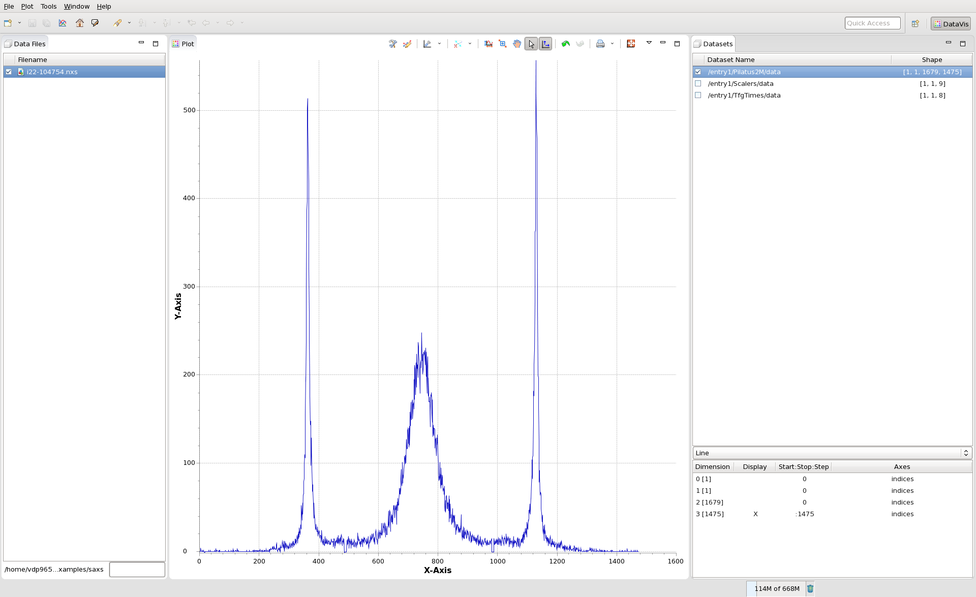
For this demo, I will load a NeXus file from data/example/saxs in the workspace. The DataVis perspective will show the name of the loaded data in the Data Files View:
When a file in this view is selected, like so:
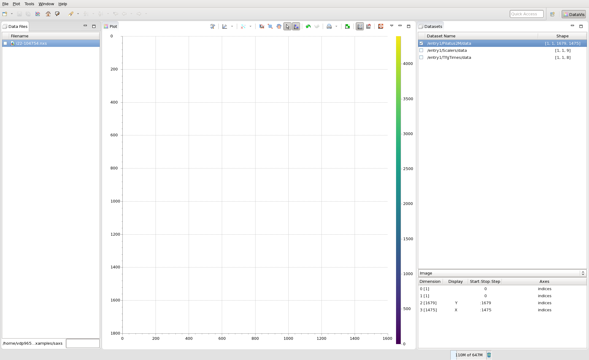
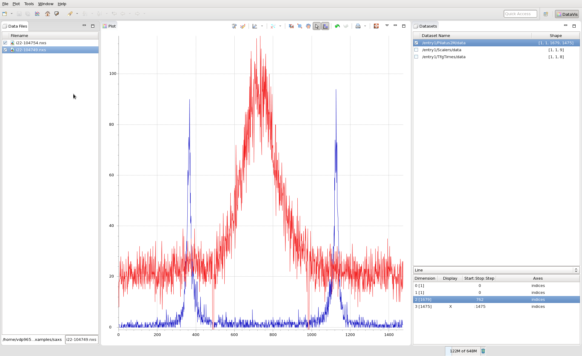
The data from the file that can be plotted (not single values, not strings like file paths, scan commands etc), will be displayed in the Datasets view:
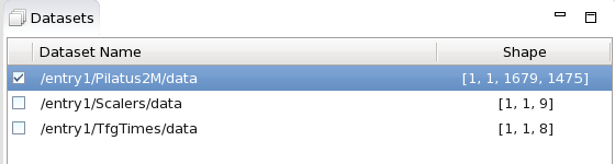
DataVis will do its best to guess what data you want to plot from the file and select it for you (e.g. the Pilatus2M data here).
The pane at the bottom of the Datasets View shows how this dataset will be dispayed (Line, Image...) and how it is currently being sliced for display.
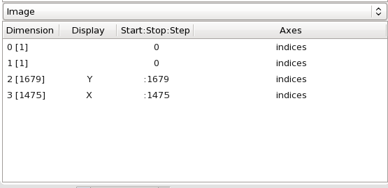
In this case, it is identified that this data should be displayed as an image, using all of the last two dimensions of the [1, 1, 1679, 1475] dataset.
At the moment no data is being displayed because the check box next to the file name in the Data Files view is not checked. Checking this box should show the image.
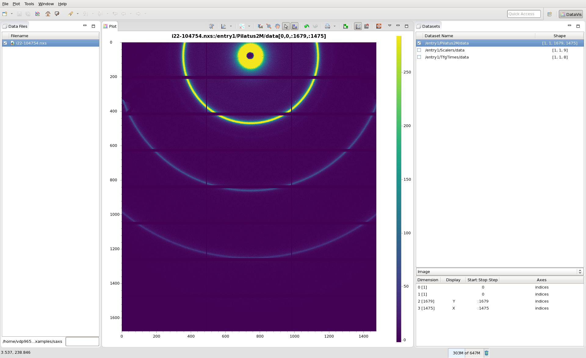
How the image looks will be very much dependent on the default colormap and histogram settings (histogram setting can be adjusted using the Quick Histogram Widget.
Viewing and Slicing Data
Now lets assume that this data is better viewed as a series of lines rather than an image.
In the pane at the bottom of the Datasets View, change Image to Line.
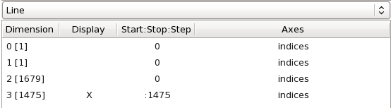
The image should be removed from the plot, and be replaced by a single line trace.
DataVis has defaulted to plot the last dimension of the data (Dimension 3, size 1475) along the X axis and it is plotting the first (0) values from Dimension 2 (size 1679).
If you want to see a different channel of the detector, click on the Start:Stop:Step column for the Dimension 2 and change the value from 0 to another number (either by manually entering the number or by using the slider).
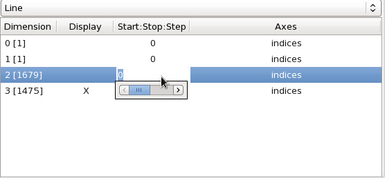
Notice how the plotted data changes.
Say you wanted to see the first 5 channels. Again click in the table cell and enter 0:5 and then press enter. 5 lines should now be plotted. Clicking again on this cell and dragging the slider will change the 5 channels displayed.
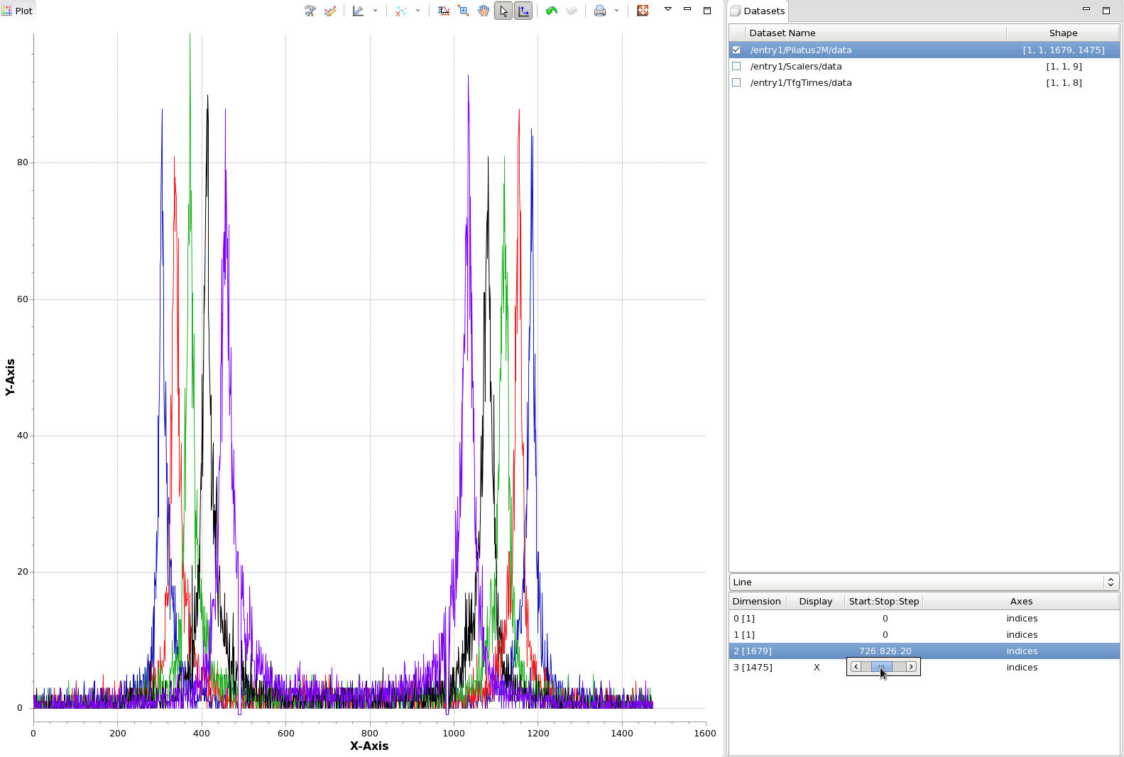
If instead you would like to see 5 samples from the first 100 channels, again click on the cell and enter 0:100:20 (hence why this column is called "Start:Stop:Step"). You should now see a different 5 lines plotted. Again dragging the slider will change the Start and Stop values.
If instead you wanted to display Dimension 2 along the X axis, Click in the Display column of the Dimension 2 row and select X from the drop down. Notice how the plotted data changes.
The Start:Stop:Step slicing also works along the dimension selected for the X axis. Say you only wanted to see the first 100 values, enter 0:100 in the Start:Stop:Step column that has X in the Dimension row. See how the plotted data changes.
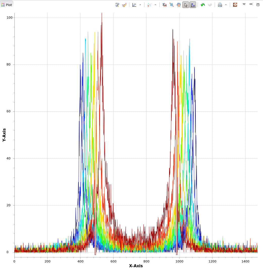
When multiple lines are plotted, they can be normalised or staggered using the options in Plot, Plot Modifiers on the main menu bar and the Quick Line Plot Offset Widget.
The colour of the lines can be changed using Plot/Line Plot Colours and selecting the colour map to apply to the sequence.
Comparing Data From Multiple Files
DataVis was designed with comparing data in mind. Say you have loaded the Pilatus image above, sliced it as a line, and found one of the channels doesn't look right, and you want to compare it to the same channel in a different image.
First lets load another file. In the same folder there was another NeXus file containing a Pilatus image of the same name and shape.
This time we will use a slightly different approach to load the data. At the bottom of the Data Files view is a label (that should show the directory containing the last file loaded) and a text box. Typing in the text box will filter against all the files in the directory, giving you options of data to load.
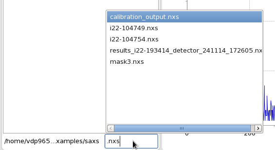
Selecting a file and pressing enter will automatically put the selected file in the text box. Pressing enter again will load the file. The text box also supports wildcards, for example entering *.nxs will load all the NeXus files in the directory. The directory this widget looks at is always the directory that contains the last file opened.
For the data being investigated here, typing part of the scan number (749.nxs) and pressing enter twice opens a new nexus file.
By default, checking the box next to this file remove the line plot (and unchecks the box next to the original file) and plots the 2M image from the new file. In this case, this is not what we want, since we want to compare two channels from the different image. We could just plot the image, change it to a line, find the same channel and then check the original file as well (multiple line plots from multiple files can be shown at once), but that is a lot of steps.
Instead, if you select the original file, Right Click and select Apply To All, this will select the same dataset and apply the same slicing to all the loaded files (that have compatible datasets).
Checking the box next to the newly loaded file should now plot the same channel from the two files over the top of each other.
Data With Axes
It is more common that not that data only makes sense when plotted against a set of axes. The images we have looked at so far have no axes, so lets load some new data and see how DataVis works with axes.
Either unload the Pilatus images or un-check the boxes to remove them from the display.
For this example a .dat file from the example data is used (315029.dat). Open it using the Recent Places link to the workspace, its in data/examples.
This file contains a stack of Pilatus images (feel free to plot, slice and investigate them), and several other datasets. In this example we shall be plotting the sum against eta.
Check the box next to the sum dataset. DataVis guesses this should be plotted as a line, with the X axis as the index to the sum array (0 to 40). Check the box next to the file name in the Data Files View to see the data plotted like this.
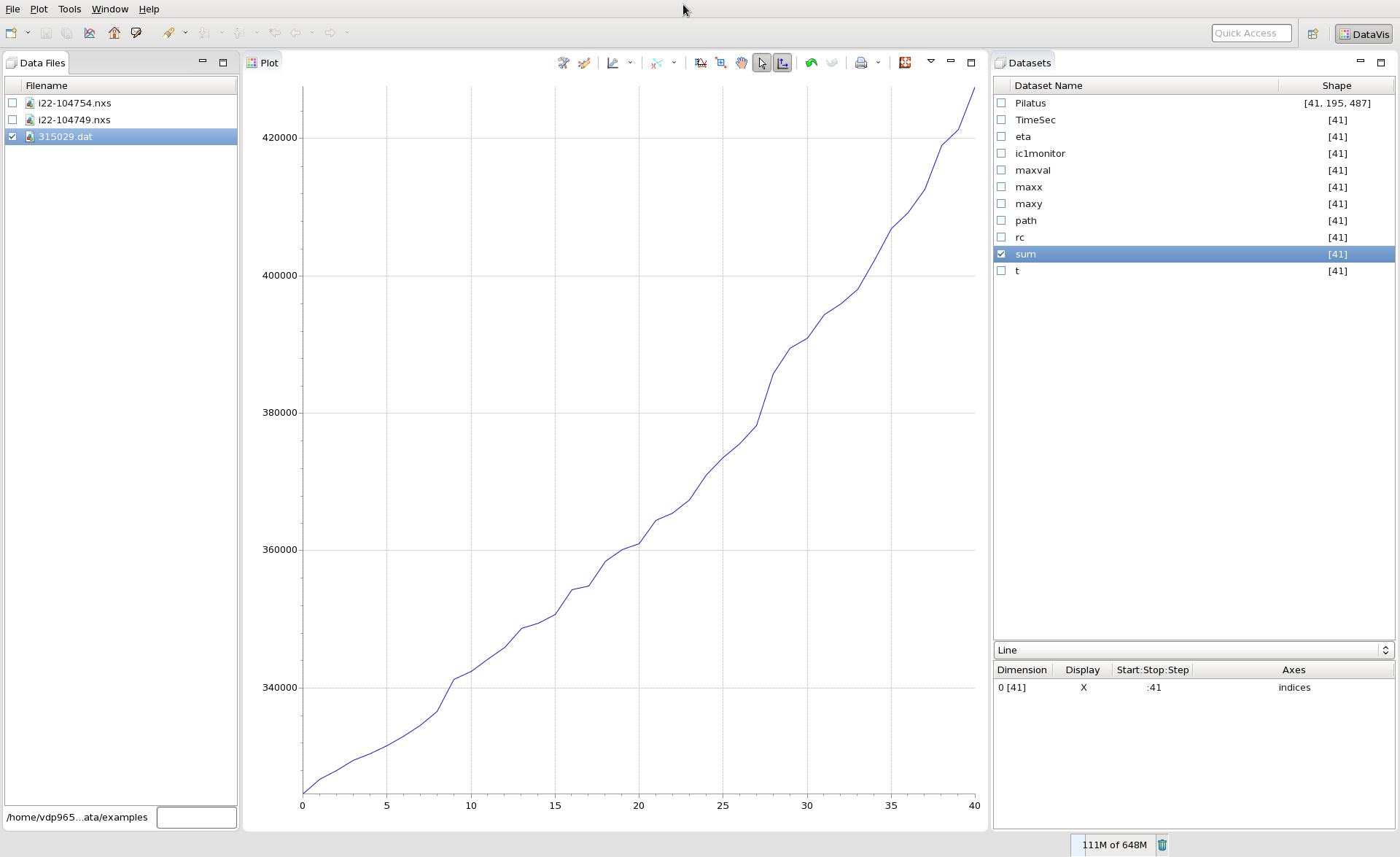
This is not what we want. The index is not the correct axis to view this data against, it should be eta. We are aiming to improve this, but there is nothing in the file to flag sum as the dataset to plot and eta as the axis to plot it against. For other file formats (NeXus for example) axes can be specified and in this case will be automatically used.
To manually change the axes, go to the widget at the bottom of the Datasets view and in the Axes column click on the cell where it says indices and change it to eta. The plot should now show sum vs eta.